

[WITH CODE] Data transformations: Time series preparation
The hidden statistical problems inside untransformed market series

Table of contents:
Introduction.
Why transform data?
The risks of data transformation.
The memory dilemma and distributional shifts.
The fractional differencing paradigm.
Higher moments and the Cornish-Fisher expansion.
Time and variance.
Time deformations and information clocks.
Structural volatility standardization.
Cross-sectional geometry and noise mitigation.
Entropy-based outlier mitigation without information loss.
Cross-sectional orthogonalization.
Non-linear embedding and phase-space reconstruction.
The unified pipeline.
Before you begin, remember that you have an index with the newsletter content organized by clicking on “Read the newsletter index” in this image.

Introduction
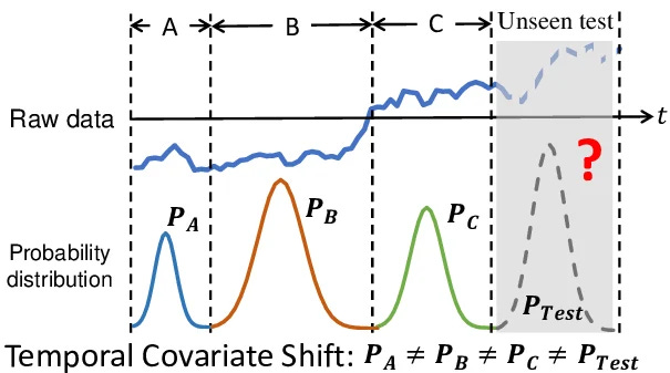
Raw market data is the closest thing we have to the market’s observable dynamics, so the instinct to leave it untouched feels sensible. But predictive models consume numerical representations. Between the tape and the optimizer there is always a translation step, whether explicit or hidden, and that translation determines which structures remain visible, which ones are attenuated, and which ones disappear. In financial machine learning, representation is part of the model itself. Prices, returns, clocks, scales, and cross-sectional coordinates all define different statistical objects, and each one presents a different geometry to the learning algorithm.
The literature on volume clocks showed that market activity is better understood in an event-driven metric than in a chronological one. The literature on fractional differencing showed that differencing need not be an all-or-nothing choice, but can instead vary continuously to preserve long-range structure while moving toward stationarity. The literature on conditional heteroskedasticity showed that variance itself has memory and must be modeled as a dynamic object rather than treated as a fixed nuisance parameter.
Here an old one about volume clock:
Yet every transformation carries a cost. A bad transformation can alter the topology of the series, flatten its tails, suppress its regime structure, and leak future information into the past. The goal here is to show that each transformation answers a specific failure mode of financial data. Some methods regularize the clock. Others preserve memory while controlling non-stationarity. Others stabilize conditional variance, correct tail asymmetry, reduce cross-sectional noise, or reconstruct hidden structure from a single observable. When these operations are applied in the right order, transformation stops being a destructive preprocessing ritual and becomes a way of making market structure legible to statistical and machine-learning models.
This is the real question is “how to make data look cleaner, but how to modify it without amputating the very dependencies we hope to trade.”
Why transform data?
If raw data represents the perfect economic reality of the market, why do we need to transform it at all? Why not feed the raw sequence of events, the actual execution prices and sizes, directly into our predictive algorithms?
The answer lies in the rigid constraints of linear algebra and numerical optimization. Machine learning algorithms, from basic Ordinary Least Squares to stochastic gradient descent solvers, don’t understand economics, market microstructure, or the concept of fiat currency. They only understand geometry and topology. They evaluate the distance between points in a high-dimensional space.
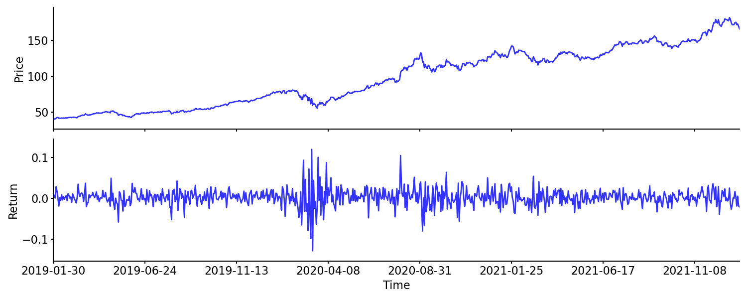
Let X∈RTxN be a feature matrix of raw asset prices over T time steps for N assets. Raw prices are strictly non-stationary I(1) processes, their mean and variance scale continually with time. If we attempt to fit a linear model to minimize the empirical risk, we must compute the inverse covariance matrix (XTX)-1 to solve for the coefficient vector. Because the raw prices share a common, unbounded macro trend, the vectors in X are collinear. The matrix XTX becomes nearly singular. Its condition number explodes, meaning the matrix inversion becomes numerically unstable. The optimizer can’t find a unique global minimum. Instead, it yields spurious regressions. The model will report a massive R2X value and highly significant t-statistics, suggesting it has found a relationship, when in reality, it has correlated two independent random walks that happen to drift in the same general direction.

Furthermore, deep learning architectures—specifically Recurrent Neural Networks and Long Short-Term Memory networks—require bounded, zero-centered inputs to propagate gradients efficiently through time. If we feed raw, un-scaled prices into a network utilizing sigmoid or hyperbolic tangent (tanh) activation functions, the architecture breaks down immediately. If an asset’s price has drifted from $10 to $400 over a decade, feeding the value $400 into a tanh function yields an output that is computationally indistinguishable from $1.0. The local derivative of the activation function at this asymptote is zero. When the backpropagation algorithm attempts to calculate the chain rule to update the network’s weights, it multiplies by this zero derivative, causing the vanishing gradient problem. The network stops learning on the very first epoch. The weights freeze.

The risks of data transformation
For some models transformation is a necessity, however it is the highest-risk component of the entire pipeline. Every operation applied to a temporal series acts as a filter. Applying an operator T(·) to a raw series Xt involves a manipulation of entropy. You are altering the properties of the dataset. If the transformation isn’t an exact bijection tailored to the specific distributional properties of the underlying asset, it is a destructive process that deletes alpha.
The primary risk is geometric distortion. Quants attempt to force non-Gaussian market data into Gaussian topologies using standardized scalers. Let μt and σt be the rolling mean and standard deviation. The standard Z-score transformation is Zt = (Xt - μt) / σt. This operation is ubiquitous in basic data science, but it is catastrophic in finance. As established by empirical market data, equity returns exhibit severe negative skewness and massive excess kurtosis. By applying this linear transformation, we assume the data is symmetric around the mean. We geometrically compress the left tail and stretch the right tail. When the optimizer processes Zt, it assigns incorrect probabilistic weights to the downside risk. The transformation has lied to the algorithm about the probability of ruin, mapping a 6σ market crash into a normalized space that makes it look like a mild, acceptable deviation.
The second critical risk is information destruction via arbitrary numerical thresholds. Common quantitative practices like hard-clipping outliers or dropping low-volume trading hours manually alter the sequence of the time series to make the data cleaner for the optimizer. If a quant runs a standard Winsorization protocol and drops an outlier return of -12% down to a hard cap of -3% simply because the extreme value “ruins the scale of the loss function,” they have committed a severe theoretical error. They have deleted the exact moment of maximum market inefficiency. That -12% print is the precise data point where algorithmic alpha is generated. It represents a moment where traders capitulated and forced liquidations occurred. Transforming the data to make it look smooth and continuous for an optimizer strips out the true signal, leaving behind highly stationary, useless white noise.
The third, and most fatal, risk is structural data leakage, also known as look-ahead bias. This occurs when a transformation operator inadvertently uses information from the future to scale or center the data of the past. If a quant runs a Principal Component Analysis (PCA) on the entire matrix X spanning from 2010 to 2024 to find orthogonal risk factors, and then trains a predictive model sequentially on the data from 2015, the model is compromised. The eigenvectors calculated by the global PCA contain variance data from the 2020 pandemic market crash. The transformation has leaked future volatility structures into the historical training set.
This leakage happens with basic functions like global mean subtraction or min-max scaling if the boundaries aren’t rolling. The model will appear profitable during out-of-sample backtesting because the transformed features implicitly “know” the future basis vectors and maximum bounds of the market. In live trading, where the production operator only has access to historical data up to time t, this false performance collapses instantly.
The memory dilemma and distributional shifts.
The fundamental dilemma in quantitative modeling revolves around the requirement for stationarity and the predictive requirement for memory. To train any robust inferential model, whether a vector autoregression or a neural architecture, the input data must be stationary. The statistical properties of the series—mean, variance, and autocorrelation structure—can’t vary over time. If they do, the model learns a regime that ceases to exist the moment it is deployed in live trading.
When you feed non-stationary price levels into a learning algorithm, you violate the core assumptions of the optimizer. As previously mentioned, in linear models like Ordinary Least Squares, non-stationarity leads to spurious regressions where the model identifies high R2 values and significant t-statistics between independent random walks. In deep learning architectures like Recurrent Neural Networks, non-stationary variance causes the gradient descent process to either vanish into zero or explode to infinity, preventing convergence.
However, the standard mathematical transformations used to enforce this required stationarity destroy the predictive power of the dataset. Financial time series, specifically price levels, are mostly I(1) processes, meaning they possess a unit root. The conventional approach to solving this is applying an integer differentiation, calculating the first-order difference or the standard log-return. This transformation achieves stationarity, yielding a series with a constant mean and finite variance. Yet, it erases the long-term memory of the process. Prices retain the entire history of market shocks, but returns only remember the shock of the immediately preceding period. By integer differencing, we obtain stationary noise that is impossible to predict.
Furthermore, integer differencing often leads to over-differencing. When you subtract Xt-1 from Xt to create a return series, you inject a moving average MA(1) component with a coefficient of -1 into the resulting noise. This artificially creates a strong negative autocorrelation at the first lag. Algorithms trained on this over-differenced data will discover short-term mean reversion that doesn’t exist in the market microstructure, leading to systematic trading losses.
The risks of relying on models built atop these conventional transformations are severe. We force non-stationary data through linear, memoryless filters, creating an illusion of predictability. We evaluate stationarity using binary heuristics like the Augmented Dickey-Fuller test, treating it as an absolute state rather than a continuous spectrum. Models trained on first-differenced data often exhibit high backtest performance due to noise-fitting but fail rapidly out-of-sample because the underlying structural dependencies of the market have been severed.
Do you rememenber the Quant Meltdown? Statistical arbitrage funds, operating with massive leverage, relied on mean-reversion models trained on orthogonalized, first-differenced equity returns. These models assumed that the residuals of their transformations were stationary, memoryless white noise, safely confined to narrow bands. When sudden, massive liquidations hit the market due to subprime mortgage exposure, the assumed independence of these time series broke down.
The residuals exhibited extreme, long-term memory. A portfolio liquidation creates a directional order flow imbalance that persists across days, resurrecting the unit root that the quants thought they had differenced away. The standard transformations had hidden it under normal, high-liquidity market conditions. When the regime shifted, the models failed because the foundation of their data transformation was inadequate. The algorithms kept doubling down on mean-reverting bets while the market displayed a persistent, memory-driven structural break.
The fractional differencing paradigm
We must abandon the misconception that differentiation is an integer operator. In the context of trading, forcing a time series into either a raw price format (where d=0) or a returns format (where d=1) is an arbitrary constraint. The correct approach is to treat differentiation as a continuous domain operator, allowing us to find the exact fractional value of d that achieves stationarity while preserving the maximum possible amount of memory.
We define the backshift operator B such that BXt = Xt-1. For any real number d, the fractional difference operator (1-B)d can be expanded using the infinite binomial series:
This expansion yields an infinite sequence of weights ωk that we apply to past observations.
Notice the recursive property of these weights:
When d=1, the math is trivial: ω0=1, ω1=-1, and all subsequent weights are zero. This describes the standard first-order difference. The memory of the series is truncated at one period.
But consider what happens when d is a fraction, say 0.5. The sequence of weights becomes ω0=1, ω1=-0.5, ω2=-0.125, ω3=-0.0625, and so on. The weights decay asymptotically to zero rather than abruptly terminating. This means Xt is transformed using an exponentially decaying window of its entire history. The current value of the transformed series is heavily influenced by yesterday’s price, moderately influenced by last week’s price, and influenced by the price a year ago. This try to mirror the market information dissemination.
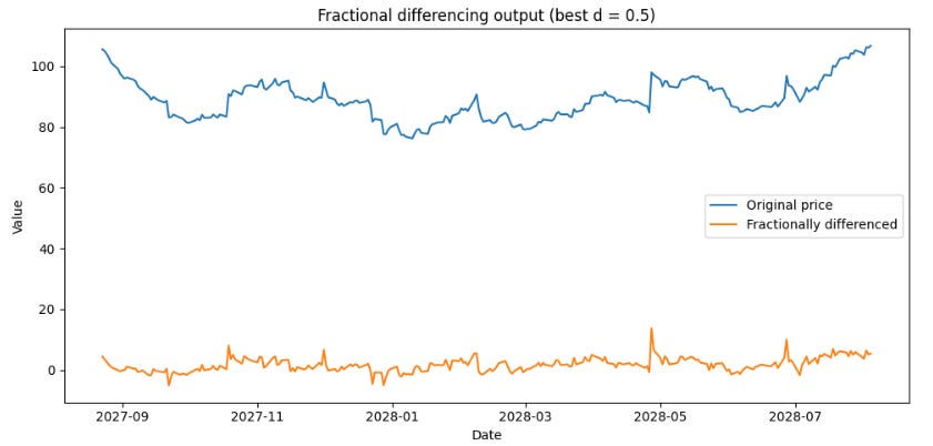
In practice, financial time series like equity indices or major fiat currencies achieve ADF stationarity at d values ranging between 0.3 and 0.4. This is an empirical fact. It proves that by using standard log-returns (d=1), the quantitative finance industry is discarding 60% to 70% of the useful memory contained in the price data.
To implement algorithm, we calculate the weights iteratively and apply a fixed-width window to prevent data leakage and memory overflow. We establish a tolerance threshold τ (often set to 10-4 or 10-5) and drop weights where |ωk| < τ. This generates a fixed lookback window, typically spanning a few thousand observations depending on the chosen threshold.
We must use a fixed-width window rather than an expanding window. If we apply fractional differencing using the entire available history of the series starting from t=0, the number of weights applied to the current observation grows as time progresses. This causes the variance of the transformed series to drift, violating the finite variance requirement of stationarity. The fixed-width window ensures that the exact same mathematical operation is applied to every observation, maintaining a constant variance profile.
Let’s implement this.
import numpy as np
import pandas as pd
from statsmodels.tsa.stattools import adfuller

def get_weights_ffd(d, length, threshold=1e-5):
    """
    Calculate weights for fractional differentiation using a fixed-width window.
    Weights iteratively decay, preserving continuous memory constraints.
    """
    weights = [1.0]
    k = 1
    while True:
        weight_k = -weights[-1] * (d - k + 1) / k
        if abs(weight_k) < threshold and k >= length:
            break
        weights.append(weight_k)
        k += 1
        if k > 10000:  # Safety break for massive arrays
            break
    return np.array(weights[::-1])

def fractional_diff(series, d, threshold=1e-5):
    """
    Applies fractional differencing to a pandas Series to maintain memory
    while achieving strict mathematical stationarity.
    """
    weights = get_weights_ffd(d, length=1, threshold=threshold)
    width = len(weights) - 1

    df = pd.Series(index=series.index, dtype=float)

    # Apply the dot product across the fixed-width rolling window
    for i in range(width, len(series)):
        window = series.iloc[i - width : i + 1]
        df.iloc[i] = np.dot(weights, window)

    return df.dropna()

def optimize_fractional_d(series, d_range=np.arange(0.1, 1.0, 0.1), p_value_threshold=0.05):
    """
    Finds the minimum fractional d that successfully passes the Augmented
    Dickey-Fuller (ADF) test for stationarity, maximizing retained memory.
    """
    for d in d_range:
        diffed = fractional_diff(series, d)
        if len(diffed) > 10:
            adf_stat = adfuller(diffed, maxlag=1, regression='c', autolag=None)
            if adf_stat[1] < p_value_threshold:
                return d
    return 1.0
This gives us the orange series you see below. Do you notice the difference compared to a simple differentiation?
Higher moments and the Cornish-Fisher expansion
Quants frequently take log-returns, subtract the rolling mean, and divide by the rolling standard deviation, assuming the resulting series z follows a standard normal distribution N(0,1). Sound familiar? This is the foundation of the Z-score, a metric that is built into the base functionality of almost every data science library.
Financial returns don’t follow a Gaussian distribution, they exhibit significant skewness and excess kurtosis. Equity markets, for example, display structural negative skew, prices drop much faster than they rise due to the mechanics of margin calls, stop-loss triggering, and fear-driven liquidity vacuums. Besides, the phenomenon of volatility clustering generates excess kurtosis, creating a distribution with a sharp central peak and fat tails.
Standardizing without accounting for these higher moments leads to severe underestimation of tail risk and generates false trading signals. Consider a standard normal distribution. A 5-standard-deviation event has a probability of approximately 2.8x10⁻⁷, which translates to an expected occurrence of once every 13,800 years of daily trading. Yet, in live equity markets, 5-sigma moves happen every few years. If an algorithm feeds a raw 5-sigma Z-score into a neural network, the model interprets it as an impossible anomaly and the assigned weights will skew, breaking the loss function.
To transform a time series into a Gaussian-equivalent state, we must incorporate its empirical skewness (S) and excess kurtosis (K). We achieve this via the Cornish-Fisher expansion, which provides a framework to estimate the quantiles of a non-normal distribution based on its specific cumulants.
If Zα is the α-quantile of the standard normal distribution, the corresponding quantile Wα of our financial time series can be approximated as:
However, in feature engineering for predictive modeling, we often need the inverse transformation. We have an observed standardized return w coming from the live market, and we want to map it back to a normal variable z so that our downstream linear models and gradient descent algorithms function correctly.
We compute the rolling skewness and rolling excess kurtosis of the time series. Estimating the third and fourth moments requires significant data to achieve statistical stability, as outliers heavily distort these metrics. Therefore, the lookback window for S and K must be longer than the window used for the mean and variance—often spanning two to three years of daily data.
Once we establish stable estimates for the cumulants, we apply the inverse Cornish-Fisher expansion to normalize the data. We map the empirical quantiles of the fat-tailed data to the theoretical quantiles of the standard normal distribution.
This adjustment guarantees that a severe market shock is processed correctly by the predictive architecture. A drop that registers as a 5-sigma event in raw standard deviations might map to a much more manageable 2.5-sigma event in the Cornish-Fisher adjusted space, reflecting its true probabilistic reality in a fat-tailed environment.
import scipy.stats as stats
import pandas as pd

def cornish_fisher_transform(returns):
    """
    Normalizes higher moments (skewness and kurtosis) mapping an empirically
    fat-tailed financial series back to a strictly Gaussian space.
    """
    # Standardize the data first based on initial 2 moments
    z = (returns - returns.mean()) / returns.std()

    # In a strict ML feature engineering pipeline, we map the empirical quantiles
    # of the fat-tailed data directly to the theoretical quantiles of the standard normal distribution

    ranks = z.rank(pct=True)

    # Map back to standard normal quantiles. We use the PPF (Percent Point Function)
    normalized = stats.norm.ppf(ranks)

    return pd.Series(normalized, index=returns.index)
I admit I like this change in silhouette. In the next post, we’ll talk about changes in shapes, I have some ideas that might be quite interesting.
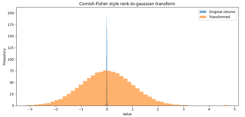
As can be seen, our distribution now looks more like a normal distribution than the classic silhouette of financial returns.
Time and variance
Data transformation involves addressing how we sample the data itself. The most pervasive obstacle in modeling financial markets is the unquestioned reliance on chronological time. Across the industry, the default behavior is to extract open, high, low, and close prices at fixed chronological intervals—minute bars, hourly bars, daily bars. This framework is a legacy artifact of print newspapers and early charting software, and it is disjointed from the reality of market micro-structure.
Market information doesn’t arrive in a continuous, uniform flow. It arrives in distinct bursts driven by human reaction and algorithmic execution. The central limit order book operates on an event-driven basis. The matching engine processes incoming FIX messages—adds, cancels, and modifications—sequentially. It has no internal concept of a “minute.” During the opening auction, or in the milliseconds following a critical macroeconomic data release like the Non-Farm Payrolls, thousands of trades occur per second. These specific moments carry massive amounts of market-moving information, representing true price discovery.
During the mid-day lull or an overnight electronic session, hours can pass with negligible volume and absolute zero new information entering the system. When we sample data chronologically, we force these disparate states into sized computational intervals. This creates a severe statistical anomaly known as a zero-inflated distribution. If you sample an illiquid asset using one-second bars, 90% of your dataset will consist of zero-returns because no trades occurred in those specific seconds. When you feed a neural network a continuous string of zero-returns, the gradient vectors collapse. The algorithm determines that the optimal prediction is always zero, stalling the learning process.
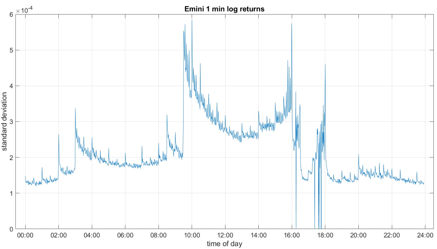
The obstacle this creates for data transformation is systemic. Chronological sampling guarantees heteroskedasticity—the variance of the data is unstable. The standard variance of a one-minute bar at 09:30 AM is an order of magnitude larger than the variance of a one-minute bar at 12:30 PM. This phenomenon creates the well-documented U-shaped intraday volatility curve. The beginning and end of the trading session contain massive variance, while the middle contains almost none.
Furthermore, chronological sampling leads to massive oversampling of low-information periods and dangerous undersampling of high-information periods. If we attempt to apply technical indicators like moving averages, momentum oscillators, or machine learning models to chronological bars, we are feeding the algorithms a distorted geometry of the market.
Time deformations and information clocks
To resolve the obstacle of chronological heteroskedasticity, we must change the domain of the temporal series. We must transition from chronological time to information time. Information can be approximated by the volume of shares traded or the total fiat value exchanged. We implement this through Time Deformations, specifically by constructing Volume Clocks or Dollar Clocks.
While some practitioners use Tick Bars (sampling every N transactions) or Volume Bars (sampling every V shares), these are suboptimal over long horizons. Tick bars are vulnerable to order fragmentation. A large institutional order sliced into 100 smaller algorithmic executions via a Time-Weighted Average Price algorithm will accelerate a tick clock without actually injecting new economic information.
You can go deeper about this kind of methods here:
![[WITH CODE] Data: Tick, Dollar and Volume bars](https://substackcdn.com/image/fetch/$s_!AJt2!,w_140,h_140,c_fill,f_webp,q_auto:good,fl_progressive:steep,g_auto/https%3A%2F%2Fsubstack-post-media.s3.amazonaws.com%2Fpublic%2Fimages%2F5cedd76e-1949-481c-a904-be1a249336c5_1280x1280.png)
Volume bars are better but remain vulnerable to corporate actions like stock splits or long-term price appreciation. Consider a multi-year backtest on a high-growth technology equity. A 10,000-share bar of a stock trading at $10 in year one represents $100,000 of market participation. If that same stock appreciates to $200 by year five, a 10,000-share bar now represents $2,000,000 of market participation. By using volume bars, the implicit information threshold has unknowingly shifted by a factor of twenty. The statistical properties of the bars from year one are incomparable to the bars from year five.
Dollar Bars correct these deficiencies, instead of sampling a new data point every time t seconds pass, we sample a new data point every time a cumulative fiat threshold θ is reached. Let vi be the volume of the i-th tick and pi be its price. The cumulative dollar volume traded at tick t is
We define the sampling times Tk such that:
When we sample the time series at these intervals Tk, we generate Dollar Bars. The threshold θ is often calculated dynamically, set to a fraction of the 50-day moving average of the daily dollar volume, ensuring the clock ticks at a consistent daily frequency even across decades of data.
The transformation from chronological space to dollar-volume space has statistical implications that directly improve model performance. Empirical studies demonstrate that the returns of dollar bars exhibit lower serial correlation. Indeed, they reduce the excess kurtosis found in chronological data. By sampling based on fiat flow, we eliminate the zero-return intervals of the overnight session and parse the massive volatility spikes of the open into multiple, manageable bars. They recover the properties of an independent and identically distributed.
By defining the series through the Dollar Clock, we adjust for both intraday seasonality and macro-regime shifts. A single Dollar Bar might span exactly 1.2 seconds during the market open, capturing the rapid influx of high-density information with perfect granularity. The subsequent Dollar Bar might span 45 minutes during the lunch hour. The variance of the returns across these bars becomes more stable.
import pandas as pd
import numpy as np
def generate_dollar_bars(ticks_df, dollar_threshold):
"""
Transforms chronological tick data into Dollar-Volume bars to eliminate
chronological heteroskedasticity.
"""
# Calculate exact fiat commitment per tick
ticks_df['dollar_value'] = ticks_df['price'] * ticks_df['volume']
ticks_df['cumulative_dollars'] = ticks_df['dollar_value'].cumsum()
# Determine discrete bar groupings based on cumulative flow
ticks_df['bar_id'] = (ticks_df['cumulative_dollars'] // dollar_threshold).astype(int)
# Aggregate raw ticks into clean OHLCV structural geometry
bars = ticks_df.groupby('bar_id').agg(
open=('price', 'first'),
high=('price', 'max'),
low=('price', 'min'),
close=('price', 'last'),
volume=('volume', 'sum'),
dollars=('dollar_value', 'sum')
)
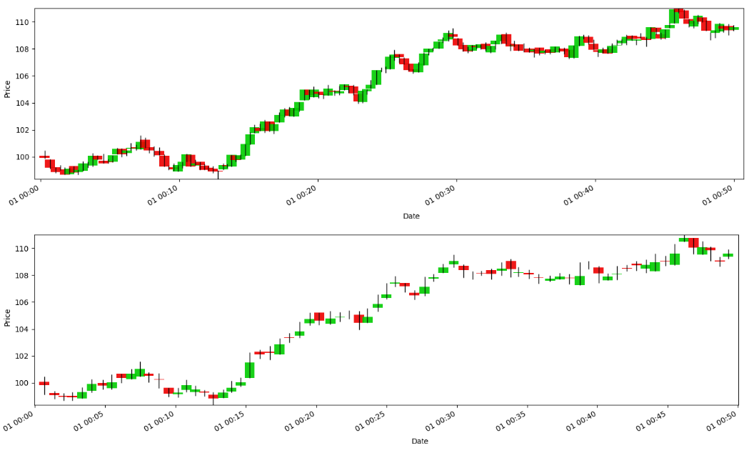
return barsLet’s take an image from one of the previous articles. If you look closely, you’ll see how sampling results in fewer bars, but also less noise.
Structural volatility standardization
Once the time series is sampled correctly using an information clock, we face the next critical transformation hurdle: volatility clustering. Even within time-deformed series, prolonged macroeconomic regimes—such as quantitative tightening cycles, global liquidity crises, or prolonged zero-interest-rate environments—cause the baseline variance of the asset to expand and contract over weeks and months. The standard quantitative practice to normalize this behavior is to standardize returns by dividing them by a simple rolling standard deviation.
This naive approach is flawed and introduces dangerous artifacts into the data matrix. A rolling standard deviation applies an equal, flat weight to all observations within the lookback window and absolute zero weight to everything outside it. Consider the exact mechanics of this operation when a massive exogenous shock enters the window. Suppose we use a 30-period rolling window. On period 1, the market drops by 10%. The estimated volatility spikes and remains elevated at a constant plateau for the next 29 periods. During this time, the true market volatility may have completely subsided, but our denominator remains massive, compressing the transformed returns and suppressing valid trading signals.
Then, exactly 30 periods later, when that specific 10% shock falls out of the lookback window, the estimated volatility drops sharply and discontinuously. This creates a mathematically induced ghost effect. The algorithm perceives a sudden collapse in market volatility, generating spurious trading signals and artificial regime shifts. A normal 0.5% return on period 31 is suddenly divided by a tiny denominator, creating a massive standardized value. In reality, absolutely nothing happened in the live market on that specific day. The anomaly was purely a structural failure of the flat rolling window equation.
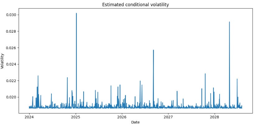
The classical transformation for volatility standardization relies on Generalized Autoregressive Conditional Heteroskedasticity ak GARCH models. Rather than relying on a flat, memoryless rolling window, we use a structural probabilistic model to estimate the conditional variance σt2 at each specific time step. For a standard GARCH(1,1) specification, the conditional variance is modeled as:
Where ε is the squared residual of the previous period (the ARCH term, representing immediate short-term market panic), and σ is the variance of the previous period (the GARCH term, representing long-term structural persistence). The constant ω defines the baseline variance level.
The power of this formulation lies in the interplay between α and β. A high α indicates a market that reacts to new information, while a high β indicates a market where volatility shocks persist for extended periods. To transform the temporal series, we fit these parameters ω, α, and β using maximum likelihood estimation over an expanding or long-term rolling window. We then filter the raw returns rt by dividing them by the modeled conditional volatility:
This GARCH-standardized series reacts to volatility because the GARCH model incorporates an exponential autoregressive decay component (β), the influence of a massive price shock diminishes over time. It never drops off a cliff. The denominator decays according to the empirical persistence of the market, eliminating the ghost effects caused by naive rolling windows.
This transformation contextualizes price action for the downstream inferential models. In a quiet market with low σt, a 2% directional move results in a value that correctly identifies an anomaly. On the other hand, in a volatile market where VIX is trading above 40, a 2% move is divided by σt.
The transformation strips out the predictable component of the volatility clustering, leaving behind a standardized, stationary residual series. It forces the predictive algorithm to focus on directional alpha of the price movement. By factoring out the structural volatility, the features fed into the final machine learning layer have a linear relationship with the future expected returns, improving the optimizer’s convergence rate.
from arch import arch_model
import warnings

def garch_standardize(returns):
    """
    Standardizes returns using structural conditional volatility estimated
    from a GARCH(1,1) model, completely bypassing the 'ghost effects'
    of naive flat rolling windows.
    """
    # Rescale returns to avoid numerical precision errors in the MLE optimizer
    scaled_returns = returns * 100

    # Define a pure volatility model assuming a zero-mean return
    am = arch_model(scaled_returns, vol='Garch', p=1, q=1, mean='Zero')

    # Fit parameters via Maximum Likelihood Estimation
    with warnings.catch_warnings():
        warnings.simplefilter("ignore")
        res = am.fit(disp='off')

    # Extract conditional volatility, scale back down, and apply standardizer
    conditional_volatility = res.conditional_volatility / 100
    standardized_returns = returns / conditional_volatility

    return standardized_returns
Remember that these are just simple examples to give you a complete picture of how and why to transform data. There are many more approaches and techniques for transforming data. In this case, if we continued with the example and used toy data, we would see something like this, and if we wanted market data, we would see something like the image above.
Cross-sectional geometry and noise mitigation
Up to this point, our transformations have focused on the isolated temporal dynamics of a single series—adjusting its memory, clock, and variance. However, institutional algorithmic trading doesn’t operate on single assets in isolation. We evaluate massive, dense feature matrices spanning hundreds of correlated instruments, exposing our optimizers to severe geometric hazards. The two most destructive issues in this cross-sectional space are the gradient-exploding impact of extreme microstructure shocks and the matrix-destabilizing curse of multicollinearity. To prepare our data for complex inferential models without erasing the underlying market signal, we must implement noise mitigation. In the following sections, we introduce two key approaches to solve outlier compression that preserves topological rank without triggering numerical overflow. Then, we apply Random Matrix Theory to orthogonally decouple and denoise the cross-sectional feature space, ensuring our covariance matrices remain mathematically stable.

Entropy-based outlier mitigation without information loss
Financial time series contain severe outliers. Broken trades, massive exogenous shocks, and unexpected central bank interventions create data points that lie far beyond the expected bounds of any standard probability distribution. Leaving these unaddressed destroys the gradient descent processes. Most optimization functions, particularly those relying on Mean Squared Error, penalize large deviations. A 10σ price shock creates a gradient update that is a hundred times larger than a standard 1σ move. If this raw data is fed into a neural network, the weights will update so violently that the model diverges, forgetting previously learned market structures.
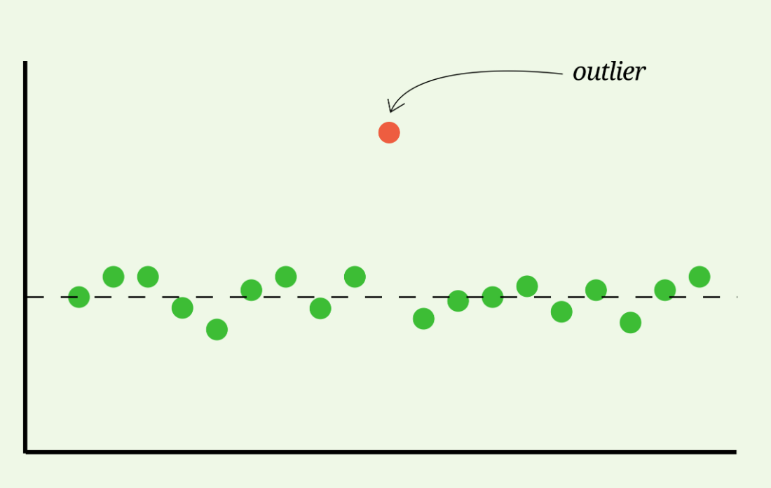
The traditional quantitative response to this problem is Winsorization: setting a static threshold (e.g., the 1st and 99th percentiles) and hard-capping any values beyond those limits. If a return exceeds the 99th percentile, it is rewritten as the 99th percentile value.
This approach is destructive and theoretically unsound. In algorithmic trading, extreme events contain the most critical alpha. Hard-capping an extreme move flattens the local gradient of the price action, deleting information about market capitulation, liquidity voids, and directional conviction. If we cap the data, a +5% move and a +15% move become identical to the algorithm. The algorithm loses the ability to distinguish between high volatility and a fundamental structural break. We need a transformation that mitigates the numerical impact of the outlier on the model’s loss function without erasing the topological information and rank order it provides.
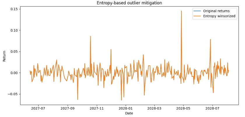
We achieve this via trimming based on Shannon Entropy. Instead of an arbitrary, static percentile, we compress the tails of the distribution using a soft-clipping function parameterized by the entropy of the rolling lookback window.
Let H(X) be the Shannon Entropy of the time series X over a recent window. We calculate this by discretizing the continuous return space into a set of B fixed bins and computing the empirical probability p(xi) of a return falling into the i-th bin:
Shannon Entropy measures the unpredictability or noise of the local market regime. If prices are bouncing randomly within a tight, mean-reverting range, the probability mass is spread across many bins, resulting in high entropy. If the market is experiencing a persistent, directional trend with low noise, the probability mass concentrates in specific bins, resulting in low entropy.
We define a threshold τ that scales inversely with this local entropy. When entropy is high (noise is elevated), the threshold tightens to compress spurious microstructure spikes. When entropy is low (a clear, persistent trend is forming), the threshold widens to capture the full magnitude of the directional move without interference.
We then apply a non-linear squashing function, the hyperbolic tangent, to the data points that exceed this dynamic τt.
Where λ controls the asymptotic limit of the compression. This entropy-based transformation acts as a differential shock absorber. The tanh function guarantees monotonicity. A +15% move will always compute to a higher transformed value than a +5% move, preserving the exact sequential logic and rank order of the time series. However, the numerical value is compressed into a safe bound (bounded by τt + λ). We preserve the exact directional information of the capitulation while neutralizing the numerical hazard that causes gradient explosion.
import numpy as np
import pandas as pd

def shannon_entropy(series, bins=50):
    """Calculates the Shannon Entropy of a time series chunk."""
    hist, _ = np.histogram(series, bins=bins, density=True)
    hist = hist[hist > 0] # Avoid log(0)
    return -np.sum(hist * np.log2(hist))

def entropy_winsorization(series, window=100, base_threshold=3.0, lambda_val=1.5):
    """
    Soft-clips outliers based on dynamic rolling entropy.
    Preserves topological information while guarding against gradient explosion.
    """
    cleaned_series = series.copy()

    for i in range(window, len(series)):
        chunk = series.iloc[i-window:i]
        entropy = shannon_entropy(chunk)

        dynamic_tau = base_threshold * (1.0 / (entropy + 0.1))
        current_val = series.iloc[i]

        if abs(current_val) > dynamic_tau:
            # Apply tanh soft clipping
            sign = np.sign(current_val)
            clipped = dynamic_tau + lambda_val * np.tanh((abs(current_val) - dynamic_tau) / lambda_val)
            cleaned_series.iloc[i] = clipped * sign

    return cleaned_series
This is starting to look more like a series that you can trade on.
Cross-sectional orthogonalization
Quants don’t usually model a single time series in isolation. It’s pretty common to evaluate dense feature matrices spanning dozens of correlated assets, hundreds of technical indicators, or entire statistical arbitrage baskets. When we transform these multiple temporal series into a unified dataset, we immediately encounter the curse of multicollinearity.
If we feed highly correlated time series—for example, the minute-by-minute returns of SPY, QQQ, and IWM—into a linear predictive model, the covariance matrix XTX becomes nearly singular. Because the vectors are almost parallel in geometric space, the determinant of XTX approaches zero. When the algorithm attempts to invert this matrix to calculate coefficients via (XTX)-1, the condition number explodes. The resulting feature weights become hyper-sensitive to microscopic noise. The model might assign a weight of +1500 to SPY and -1499 to QQQ just to fit a tiny basis point of random variance. This leads to catastrophic overfitting and immediate out-of-sample failure.
The required transformation is Cross-Sectional Orthogonalization, executed via PCA or Gram-Schmidt orthonormalization across the time domain. By transforming the raw, correlated feature space into an orthogonal basis, we geometrically decouple the variance.
Let X be our T ∈ N matrix of standardized time series. We compute the empirical covariance matrix
Because Σ is symmetric and positive semi-definite, we can perform an eigendecomposition to find the orthogonal eigenvectors W and their corresponding eigenvalues λ:
The eigenvectors represent the orthogonal directions of maximum variance in the market. The time series are then transformed into Principal Components Z:
The resulting matrix Z consists of N uncorrelated time series. The dot product of any two distinct columns in Z is zero. In quantitative finance, these components have direct, tradable economic interpretations. The first principal component (Z1), associated with the largest eigenvalue, universally represents the underlying market beta—the systemic risk factor moving all assets. The second and third components represent sector rotations, value-growth spreads, or distinct macroeconomic risk premia.
By applying this transformation, we solve the multicollinearity problem. The optimizer can now assign weights to independent risk factors. Furthermore, we leverage this orthogonalization to denoise the entire system using Random Matrix Theory, applying the Marchenko-Pastur distribution.
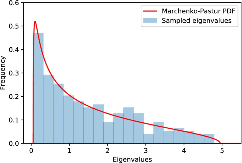
Not all computed eigenvectors contain actual signal. Eigenvectors associated with eigenvalues near zero represent idiosyncratic microstructure bounce—pure noise. According to the Marchenko-Pastur theorem, we can analytically calculate a threshold eigenvalue below which the variance is statistically indistinguishable from a random matrix.
We discard these low-variance principal components. We set their eigenvalues to zero and reconstruct the time series using only the top K components. This generates a synthetic, orthogonalized data matrix that captures the true underlying drivers of the market while deleting the highly correlated, overfitted noise. Algorithms trained on this subspace converge rapidly and display superior out-of-sample Sharpe ratios.
from sklearn.decomposition import PCA
import pandas as pd
import numpy as np
def pca_orthogonalize(df_features, variance_threshold=0.95):
"""
Transforms cross-sectional time series into orthogonal Principal Components,
filtering out multicollinearity and idiosyncratic noise.
"""
# Standardize features to ensure fair variance extraction
standardized = (df_features - df_features.mean()) / df_features.std()
# Initial fit to evaluate the variance explained by each orthogonal factor
pca = PCA()
pca.fit(standardized)
# Determine the number of principal components to keep (Marchenko-Pastur proxy)
cumulative_variance = np.cumsum(pca.explained_variance_ratio_)
n_components = np.argmax(cumulative_variance >= variance_threshold) + 1
# Re-fit and transform the data using only the strictly valid components
pca_reduced = PCA(n_components=n_components)
components = pca_reduced.fit_transform(standardized)
# Reconstruct the feature matrix in the new, uncorrelated topological space
columns = [f'PC_{i+1}' for i in range(n_components)]
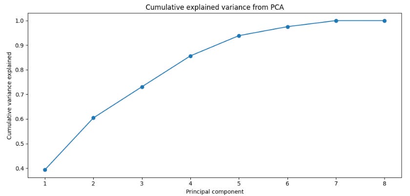
return pd.DataFrame(components, index=df_features.index, columns=columns)In this plot we can see how there are a few components that explain the variance of the data we have used.
Non-linear embedding and phase-space reconstruction
The preceding six transformations focus on structural adjustment, stationarity, and linear geometry. However, financial markets also display complex nonlinear dynamics driven by interacting algorithmic agents, endogenous liquidity feedback loops, and other factors.
In dynamical-systems terms, this behavior arises from a deterministic system with extreme sensitivity to initial conditions, a property that can be quantified through a positive maximal Lyapunov exponent. To model this kind of temporal behavior, analyzing a one-dimensional sequence x1, x2, …, xt is insufficient. The time series obtained from an exchange API is only a single observable projection of a far more complex multidimensional system.
When we track the price of an asset, we observe only one coordinate of a much larger state space. The hidden variables remain unobserved: aggregate market maker inventory, institutional limit orders resting off-book, options-driven delta-hedging pressure, and the intraday collateral constraints of leveraged funds. Since explicit measurement of all these variables is impossible, we must transform the 1D time series into a multidimensional geometric representation.
This is precisely the role of Takens’ Delay Embedding Theorem. Under broad regularity conditions, the theorem shows that a single observed time series can be used to reconstruct a geometry that is diffeomorphic, or smoothly equivalent, to the underlying hidden attractor of the full dynamical system. We don’t need direct access to the latent variables. Their influence is already encoded in the sequential history of the observable series.
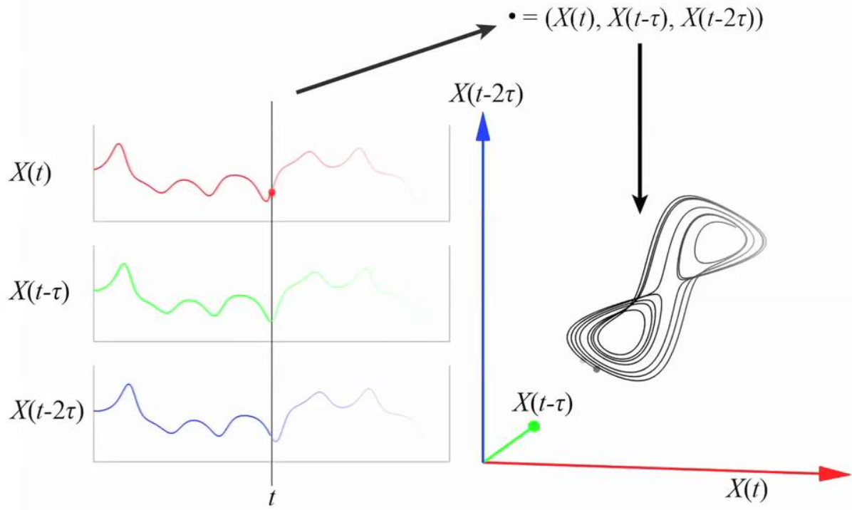
We transform the scalar time series xt into an m-dimensional vector xt using a time delay τ:
This mapping lifts the time series into phase space. The choice of the delay τ and the embedding dimension m is critical because the validity of the reconstructed geometry depends on both.
If τ is too small, the coordinates xt and xt-τ remain highly correlated, so the embedded points collapse near a diagonal and provide almost no new structural information. If τ is too large, the coordinates become nearly independent, the deterministic linkage weakens, and the reconstructed geometry loses coherence. The standard way to select τ is to compute the mutual information between xt and xt-τ across candidate lags. Unlike Pearson correlation, mutual information is entropy-based and captures nonlinear dependence. We choose the first local minimum, which identifies the delay where the next coordinate contributes maximum new structural information while still preserving dynamical dependence.
We determine the embedding dimension m through the False Nearest Neighbors algorithm. If a genuinely high-dimensional system is projected into a space of insufficient dimension, trajectories that are actually far apart can appear artificially close. The FNN procedure increases the dimension step by step. For each point, it identifies its nearest neighbor in dimension m, then measures how that same pair separates when lifted into dimension m+1. If the distance expands beyond a prescribed threshold, the neighbor was false. We stop increasing m when the proportion of false nearest neighbors approaches zero. At that point, the attractor has been properly unfolded and the geometric trajectories no longer overlap because of projection error.
Once we plot the transformed matrix X in two or three dimensions, we no longer observe a jagged price trace indexed by time. We observe the geometry of market regimes. A mean-reverting regime can generate a torus-like structure. A persistent directional regime can form a stretched manifold. A volatility expansion can appear as an outward spiral.
By transforming the time series into phase space, we allow models such as convolutional neural networks and support vector machines to analyze the data as a spatial and topological object rather than as a raw sequence of values. We can further map the embedded trajectories into Gramian angular fields. A CNN can then scan the resulting matrix as it would scan an image, learning the geometric signature of a volatil regime instead of memorizing a noisy run of negative returns. The task shifts from forecasting a scalar value to recognizing a geometric configuration.
import numpy as np
def takens_embedding(series, m, tau):
"""
Reconstructs the multi-dimensional phase space of a chaotic dynamical system
from a single 1D temporal series using Takens' Delay Embedding Theorem.
"""
N = len(series)
# Mathematical guardrail: ensure we have enough data points to populate the geometry
if N < (m - 1) * tau + 1:
raise ValueError("Time series is mathematically too short for these embedding parameters.")
# Initialize the phase-space matrix
embedded = np.zeros((N - (m - 1) * tau, m))
# Vectorized mapping of the delayed coordinates into the topological space
for i in range(m):
# We slice the array with the necessary delays and assign to the specific dimension
embedded[:, i] = series.iloc[i * tau : N - (m - 1) * tau + i * tau]
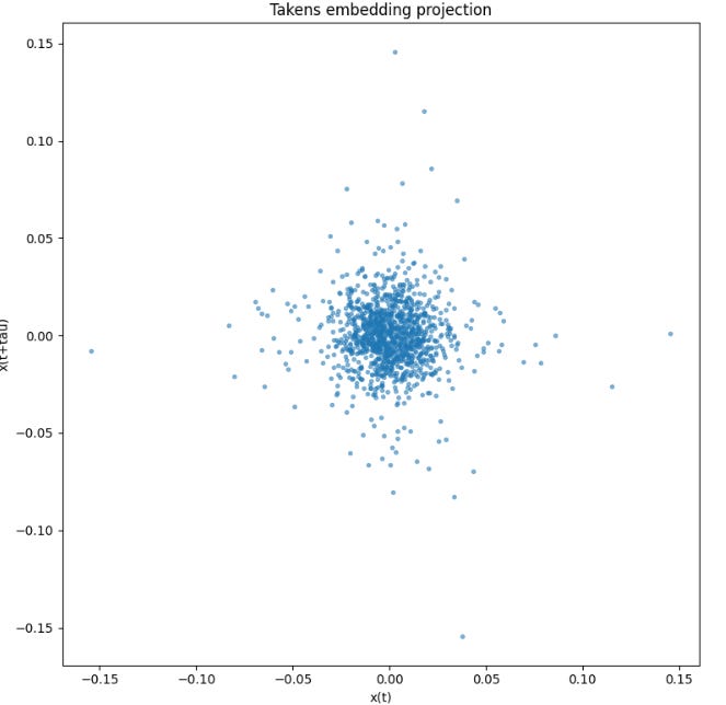
return embeddedThe reconstructed phase-space projection forms a dense cloud centered near the origin, with no clear low-dimensional manifold, closed orbit, or recurrent geometric skeleton. This suggests that, at the selected delay, the observable is dominated by noise or weak dependence rather than by a visually recoverable deterministic structure.
The unified pipeline
The core conflict of data transformation in quantitative finance lies in the attempt to apply singular, naive adjustments to a complex system. The quantitative finance industry is littered with the remnants of funds that treated data transformation as a menu of independent choices, or worse, engaged in kitchen-sink feature engineering by feeding 500 un-transformed indicators into a gradient boosting model. If a quant applies a standard scaler without adjusting for non-normality, or differentiates integer-wise without considering memory, the resulting models are doomed to fail in production.
The correct chronological execution of this pipeline resolves the fundamental obstacles:
Deformation: We first eliminate chronological heteroskedasticity by sampling the raw tick data using a Dollar-Volume clock. The series moves into information-time.
Stationarity: We apply Fractional Differencing to the dollar bars. We optimize the d parameter to achieve stationarity while maintaining the maximum theoretical memory. This step requires the stable variance profile created by the time deformation in step one.
Outlier mitigation: We apply the entropy-based soft-clipping function to neutralize extreme prints without destroying the topological footprint of the shock. We do this before volatility modeling to prevent a single extreme outlier from biasing the GARCH parameter estimation. If a extreme volatility hits a GARCH model without prior entropy clipping, the conditional variance explodes and suppresses the transformed returns for the next N periods.
Volatility standardization: We fit a GARCH(1,1) model and divide the fractionally differenced, clipped series by the conditional volatility to remove autoregressive variance clustering.
Distributional adjustment: We calculate the empirical skewness and kurtosis and apply the inverse Cornish-Fisher expansion to normalize the higher moments of the data. This must occur after GARCH standardization. GARCH removes the conditional, short-term volatility bursts, leaving behind the true, unconditional structural non-normality of the asset for the Cornish-Fisher expansion to correct.
Orthogonalization: Across multiple parallel assets, we apply PCA to extract the uncorrelated risk factors, dropping the noise-heavy eigenvectors via Marchenko-Pastur thresholding. We can only compute valid covariance matrices for PCA because the prior five steps guaranteed that our individual series are stationary, outlier-free, and distributionally stable. If you run PCA on raw returns, the principal components align with the noise.
Embedding: Finally, if required by the predictive architecture, we map the clean, stationary, orthogonalized sequence into an m-dimensional phase space using Takens’ Theorem. This topological mapping requires pristine data. Otherwise, Takens’ theorem simply maps the microstructure noise instead of the system’s actual attractor.
In a live trading environment, these seven steps must be computed sequentially on streaming tick data with sub-millisecond latency. This demands optimized C++ implementations or JAX-compiled Python arrays, bypassing the overhead of standard pandas dataframes.

Cool guys! Good job today! Remember that you have the full code in the appendix so you can torture it. Time to say good bye! Stay sharp, stay bold, stay unshakeable 📈
PS: What do you prefer to trade, big caps or small caps?
This is an invitation-only access to our QUANT COMMUNITY, so we verify numbers to avoid spammers and scammers. Feel free to join or decline at any time. Tap the WhatsApp icon below to join

Appendix
Full code:
import warnings
import numpy as np
import pandas as pd
import scipy.stats as stats
import matplotlib.pyplot as plt

from scipy.optimize import minimize
from statsmodels.tsa.stattools import adfuller
from sklearn.decomposition import PCA

warnings.filterwarnings("ignore")

class TimeSeriesTransformer:
    def get_weights_ffd(self, d, length, threshold=1e-5):
        weights = [1.0]
        k = 1
        while True:
            weight_k = -weights[-1] * (d - k + 1) / k
            if abs(weight_k) < threshold and k >= length:
                break
            weights.append(weight_k)
            k += 1
            if k > 10000:
                break
        return np.array(weights[::-1])

    def fractional_diff(self, series, d, threshold=1e-5):
        weights = self.get_weights_ffd(d, length=1, threshold=threshold)
        width = len(weights) - 1
        out = pd.Series(index=series.index, dtype=float)
        vals = series.to_numpy(dtype=float)
        for i in range(width, len(series)):
            out.iloc[i] = np.dot(weights, vals[i - width:i + 1])
        return out.dropna()

    def optimize_fractional_d(self, series, d_range=np.arange(0.1, 1.0, 0.1), p_value_threshold=0.05):
        best = None
        rows = []
        for d in d_range:
            diffed = self.fractional_diff(series, d)
            if len(diffed) > 10:
                adf_stat = adfuller(diffed, maxlag=1, regression="c", autolag=None)
                rows.append((d, adf_stat[0], adf_stat[1], len(diffed)))
                if best is None and adf_stat[1] < p_value_threshold:
                    best = d
        return (1.0 if best is None else best), pd.DataFrame(rows, columns=["d", "adf_stat", "p_value", "n_obs"])

    def cornish_fisher_transform(self, returns):
        z = (returns - returns.mean()) / returns.std(ddof=0)
        ranks = z.rank(pct=True).clip(1e-6, 1 - 1e-6)
        return pd.Series(stats.norm.ppf(ranks), index=returns.index)

    def generate_dollar_bars(self, ticks_df, dollar_threshold):
        df = ticks_df.copy()
        df["dollar_value"] = df["price"] * df["volume"]
        df["cumulative_dollars"] = df["dollar_value"].cumsum()
        df["bar_id"] = (df["cumulative_dollars"] // dollar_threshold).astype(int)
        return df.groupby("bar_id").agg(
            open=("price", "first"),
            high=("price", "max"),
            low=("price", "min"),
            close=("price", "last"),
            volume=("volume", "sum"),
            dollars=("dollar_value", "sum"),
        )

    def _garch11_negloglik(self, params, r_scaled):
        omega, alpha, beta = params
        if omega <= 1e-10 or alpha < 0 or beta < 0 or alpha + beta >= 0.999:
            return 1e12
        h = np.empty(len(r_scaled))
        h[0] = np.var(r_scaled, ddof=1)
        for t in range(1, len(r_scaled)):
            h[t] = omega + alpha * (r_scaled[t - 1] ** 2) + beta * h[t - 1]
            if h[t] <= 1e-12 or not np.isfinite(h[t]):
                return 1e12
        return 0.5 * np.sum(np.log(2 * np.pi) + np.log(h) + (r_scaled ** 2) / h)

    def garch_standardize(self, returns):
        r = returns.dropna().to_numpy(dtype=float)
        scale = 100.0
        r_scaled = r * scale
        var0 = np.var(r_scaled, ddof=1)
        x0 = np.array([0.01 * var0, 0.05, 0.90])
        bounds = [(1e-10, None), (0.0, 0.999), (0.0, 0.999)]
        constraints = ({"type": "ineq", "fun": lambda x: 0.999 - (x[1] + x[2])},)
        res = minimize(
            self._garch11_negloglik,
            x0,
            args=(r_scaled,),
            method="SLSQP",
            bounds=bounds,
            constraints=constraints,
            options={"maxiter": 500},
        )
        if res.success:
            omega, alpha, beta = res.x
            h = np.empty(len(r_scaled))
            h[0] = var0
            for t in range(1, len(r_scaled)):
                h[t] = omega + alpha * (r_scaled[t - 1] ** 2) + beta * h[t - 1]
        else:
            lam = 0.94
            h = np.empty(len(r_scaled))
            h[0] = var0
            for t in range(1, len(r_scaled)):
                h[t] = (1 - lam) * (r_scaled[t - 1] ** 2) + lam * h[t - 1]
        cond_vol = np.sqrt(h) / scale
        return (
            pd.Series(r / cond_vol, index=returns.dropna().index),
            pd.Series(cond_vol, index=returns.dropna().index),
            {"success": bool(res.success), "params": res.x if res.success else np.array([np.nan, np.nan, np.nan])},
        )

    def shannon_entropy(self, series, bins=50):
        hist, _ = np.histogram(series, bins=bins, density=True)
        hist = hist[hist > 0]
        return -np.sum(hist * np.log2(hist))

    def entropy_winsorization(self, series, window=100, base_threshold=3.0, lambda_val=1.5):
        cleaned = series.copy()
        taus = pd.Series(index=series.index, dtype=float)
        for i in range(window, len(series)):
            chunk = series.iloc[i - window:i]
            entropy = self.shannon_entropy(chunk)
            tau = base_threshold * (1.0 / (entropy + 0.1))
            taus.iloc[i] = tau
            x = series.iloc[i]
            if abs(x) > tau:
                sign = np.sign(x)
                clipped = tau + lambda_val * np.tanh((abs(x) - tau) / lambda_val)
                cleaned.iloc[i] = clipped * sign
        return cleaned, taus

    def pca_orthogonalize(self, df_features, variance_threshold=0.95):
        z = (df_features - df_features.mean()) / df_features.std(ddof=0)
        pca_full = PCA()
        pca_full.fit(z)
        cum_var = np.cumsum(pca_full.explained_variance_ratio_)
        n_components = np.argmax(cum_var >= variance_threshold) + 1
        pca_reduced = PCA(n_components=n_components)
        comps = pca_reduced.fit_transform(z)
        cols = [f"PC_{i+1}" for i in range(n_components)]
        return pd.DataFrame(comps, index=df_features.index, columns=cols), pd.Series(
            pca_full.explained_variance_ratio_,
            index=[f"PC_{i+1}" for i in range(len(pca_full.explained_variance_ratio_))]
        )

    def takens_embedding(self, series, m, tau):
        N = len(series)
        if N < (m - 1) * tau + 1:
            raise ValueError("Time series is too short for these embedding parameters.")
        embedded = np.zeros((N - (m - 1) * tau, m))
        for i in range(m):
            embedded[:, i] = series.iloc[i * tau:N - (m - 1) * tau + i * tau]
        return embedded
This is truly a very useful article, not just for reading but to put in practice.
I have a question regarding the Cornish Fisher Transform. You talk about calculating rolling skew, kurtosis, but don't see that in the code.
The transform should be applied on a rolling basis, right? Otherwise, this will create a look-ahead bias. or is this supposed to be applied like a StandardScaler for preprocessing?
Great article QB.
I have a question-- before orthogonalization, would you align all assets to the same time points by using each asset’s most recently completed bar, so every asset ends up with the same number of rows even though volume bars occur at different times?