


Table of contents:
Introduction.
Risk and limitations of time bars.
Introducing information-driven bars.
Range bars.
Renko bars.
Filter bars.
Volatility bars.
Before you begin, remember that you have an index with the newsletter content organized by clicking on “Read full story” in this image.

Introduction
You are observing the markets in real-time—thousands of price ticks cascading across your screen, each reflecting a momentary shift in supply, demand, and sentiment. At first glance, the data appears evenly spaced, structured, and regular. Yet beneath this surface lies a deeper asymmetry: the rhythm of market activity is not governed by the uniform cadence of the wall clock, but by the irregular pulses of information flow and volatility.
This distinction underscores a fundamental challenge in financial data sampling: the dissonance between chronological time and what might more aptly be termed market time. While traditional time bars—such as 1-minute or 5-minute intervals—offer simplicity and compatibility with standard backtesting frameworks, they assume that each unit of time carries equal informational weight. The reality, however, is far more complex.
Markets are event-driven. Activity and volatility are not uniformly distributed. A 5-minute interval during a low-liquidity midday lull is not equivalent to a 5-minute window during a central bank announcement. Yet both are treated identically in time-based sampling. This can lead to misleading signals, particularly for strategies sensitive to volatility regimes or order flow.
Moreover, time bars introduce well-known statistical complications. Volatility clustering results in periods of extreme variability being aggregated in the same temporal units as periods of calm, producing heteroskedastic return series that impair the performance of risk models, signal generation algorithms, and machine learning architectures. For example, attempts to train predictive models on such unevenly informative data may yield unstable or overfit outcomes.
Alternative approaches, such as tick bars, volume bars, and dollar bars, aim to address these shortcomings by redefining sampling based on market activity rather than elapsed time. Tick bars group a fixed number of trades, adapting to bursts of market engagement. Volume bars aggregate data until a fixed number of shares or contracts have changed hands. Dollar bars go further, normalizing across instruments by aggregating based on the notional value traded. These methods tend to produce more statistically stable returns and better align with the flow of market information. Check about these bars here:

Ultimately, selecting an appropriate sampling method is not a matter of convenience—it is a design decision that shapes the behavior, accuracy, and robustness of a trading strategy. While time-based bars remain common, their limitations should not be overlooked. Today we'll be reviewing a completely different type of bar, some of which are quite common and popular among traders.
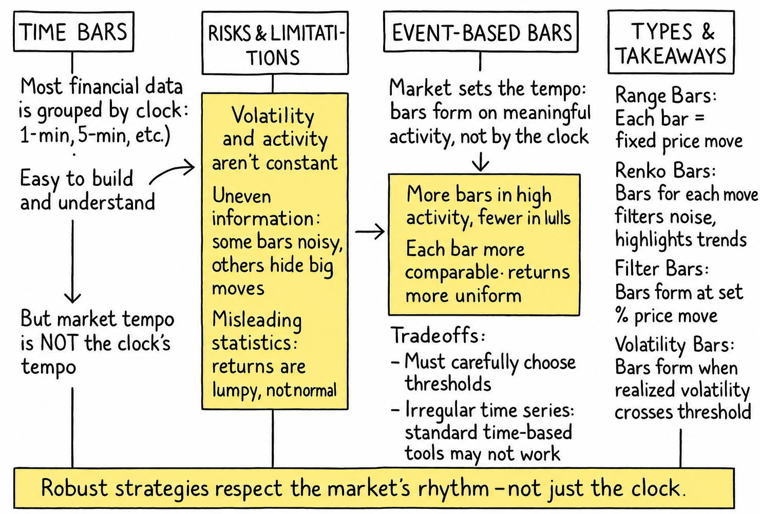
Risk and limitations of time bars
Moving beyond time-based bars is a quest for a more intelligent market clock, one that ticks not with the passage of seconds, but with the occurrence of meaningful events. The idea is to sample observations not when the clock dictates, but when the market does something interesting. This leads us to the concept of information-driven bars, where each bar represents a consistent quantum of information, however that might be defined–a certain price movement, a specific volume traded, or a particular amount of capital changing hands.
But this path is no sunlit meadow; it is a labyrinth, riddled with multiple obstacles. The very flexibility that makes these bars appealing also introduces complexity.
How much price movement constitutes a "meaningful event"?
How large should a "brick" of price change be?
What level of volatility warrants a new bar?
These questions throw the algorithmic trader into the murky waters of parameter selection, a domain where the siren song of overfitting constantly plays. Furthermore, the irregular arrival of these bars in clock time can make traditional time-series analysis techniques more challenging to apply directly, requiring new perspectives on concepts like duration and seasonality.
Traditional time-based bars—e.g., 1-minute, 1-hour—are the historical default. They sample price data at fixed temporal intervals. While simple to compute and understand, their core flaw lies in the assumption that market activity is uniformly distributed across time. This is demonstrably false. Markets exhibit periods of high and low activity, and time-based bars treat these identically.
Consider two 5-minute bars:
Bar A (low activity): Price meanders within a tight range. The bar captures minimal information, potentially just noise.
Bar B (high activity): A news event causes price to surge and plummet. The bar captures a significant trend and volatility, but crams it into the same temporal box as Bar A.
This disparity leads to several issues for algorithmic models:
The variance of returns is not constant across bars. Statistical models assuming homoskedasticity will be misspecified.
The distribution of returns from time-based bars often exhibits excess kurtosis—fat tails—and skewness, deviating from the normal distribution assumed by many financial models.
During low activity, time bars accumulate noise. During high activity, crucial intraday details within the fixed interval can be lost or averaged out.
The illusion is that we are measuring the market; in reality, we are often just measuring the clock, forcing market behavior into an arbitrary temporal grid. The quest, therefore, is to find sampling methods that adapt to the market's rhythm, not an external one.
Introducing information-driven bars
Information-driven bars, or event-based bars, are constructed based on the flow of information rather than the passage of time—What matters here is what we consider information.. The goal is to create bars that each represent a similar amount of "market eventfulness." This synchronicity aims to produce a bar series with more desirable statistical properties, such as returns that are closer to being independently and identically distributed and, ideally, closer to a normal distribution.
The fundamental premise is that significant market events—price changes, volume surges, volatility spikes—are what truly matter. By forming bars based on these events, we let the market itself dictate the sampling frequency. When the market is frenetic, bars form rapidly, capturing the action. When the market is placid, bars form slowly, patiently waiting for meaningful information. This dynamic sampling is the hallmark of price-movement bars.
The following Python snippet outlines a base class structure that has been developed by Hudson and Thames and we are going to use to build all the bars. Furthermore, it can be used to implement various types of information-based toolbars, not just those popularized by López de Prado. This illustrates the common framework before diverging into specific event triggers.
from abc import ABC, abstractmethod
import pandas as pd
import numpy as np
from collections import deque

def _batch_chunks(df, size):
    """
    Split DataFrame into equal-sized chunks for batch processing.
    """
    idx = np.arange(len(df)) // size
    return [grp for _, grp in df.groupby(idx)]


class BaseBars(ABC):
    def __init__(self, metric=None, batch_size=int(2e7)):
        self.metric = metric
        self.batch_size = batch_size
        self.reset()

    def reset(self):
        self.open = self.high = self.low = self.close = None
        self.prev_price = None
        self.tick_rule = 0
        self.stats = dict(cum_ticks=0, cum_dollar=0, cum_vol=0, cum_buy_vol=0)

    def _sign(self, price):
        if self.prev_price is None:
            diff = 0
        else:
            diff = price - self.prev_price
        self.prev_price = price
        if diff != 0:
            self.tick_rule = np.sign(diff)
        return self.tick_rule

    def run(self, rows):
        bars = []
        for t, p, v in rows:
            self.stats['cum_ticks'] += 1
            self.stats['cum_dollar'] += p * v
            self.stats['cum_vol'] += v
            if self._sign(p) > 0:
                self.stats['cum_buy_vol'] += v
            # initialize OHLC
            if self.open is None:
                self.open = self.high = self.low = p
            # update
            self.high = max(self.high, p)
            self.low = min(self.low, p)
            self.close = p
            # check threshold
            self._check_bar(t, p, bars)
        return bars

    def batch_run(self, data, to_csv=False, out=None):
        cols = ['date', 'tick', 'open', 'high', 'low', 'close',
                'vol', 'buy_vol', 'ticks', 'dollar']
        bars = []
        if isinstance(data, pd.DataFrame):
            chunks = _batch_chunks(data, self.batch_size)
        else:
            chunks = pd.read_csv(data, chunksize=self.batch_size, parse_dates=[0])
        for chunk in chunks:
            bars.extend(self.run(chunk[['date', 'price', 'volume']].values))
        df = pd.DataFrame(bars, columns=cols)
        df['date'] = pd.to_datetime(df['date'])
        df.set_index('date', inplace=True)
        if to_csv and out:
            df.to_csv(out)
        return df

    @abstractmethod
    def _check_bar(self, t, p, bars):
        ...
This BaseBars class elegantly provides a common engine for accumulating tick data and delegates the crucial decision of when to form a bar to its children. This is the dawn of designing our own market clocks.

Range bars
Range bars are among the conceptually simplest price-movement bars. A new bar is formed when the price range (High - Low, or more commonly |Close - Open| of the forming bar) exceeds a predefined threshold, R.
The condition to close a RangeBar k when observing tick i is:
where openk is the open price of the current bar being built, and closei is the current tick's price.
The allure of range bars is their promise of uniformity in price movement per bar. Each bar, by definition, represents a price journey of at least R. This can help normalize price fluctuations, making subsequent analyses like volatility estimation or pattern recognition more consistent.
If you'd like to dig a little deeper, check out this PDF. I liked its approach:
Here's how the RangeBars class implements this logic, inheriting from BaseBars:
class RangeBars(BaseBars):
    def __init__(self, threshold, batch_size=int(2e7)):
        super().__init__(None, batch_size)
        self.threshold = threshold

    def _check_bar(self, t, p, bars):
        if self.open is None:
            return
        if abs(self.close - self.open) >= self.threshold:
            bars.append([pd.to_datetime(t), self.stats['cum_ticks'],
                         self.open, self.high, self.low, self.close,
                         self.stats['cum_vol'], self.stats['cum_buy_vol'],
                         self.stats['cum_ticks'], self.stats['cum_dollar']])
            self.reset()
The _check_bar method is the heart here. Once the price stretches sufficiently from its opening point, a bar is "born," and the process resets, waiting for the next R-sized journey. The challenge, of course, is choosing an appropriate R. Too small, and you're swamped with noisy bars. Too large, and you miss crucial subtleties.
Let’s see:
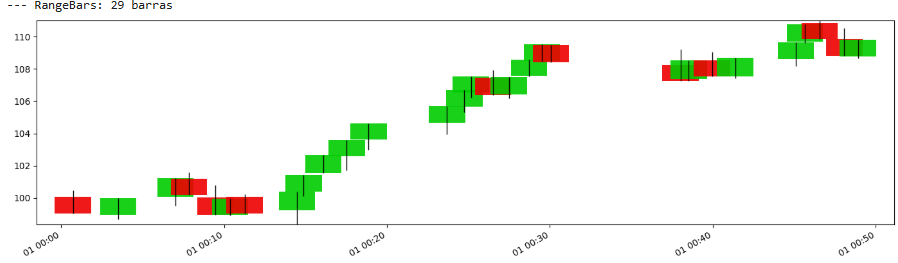
During high volatility, many such bars would form in a short clock-time period, while in low volatility, fewer bars would form over a longer clock-time period.
Advantages:
Each bar—ideally—represents a consistent amount of price excursion. This can help normalize price action.
More bars will form during periods of high price movement—volatility—and fewer during quiet periods, naturally focusing sampling where the action is.
The fixed range can sometimes help in identifying mini support and resistance levels defined by the range quantum R.
By requiring a minimum price movement, some of the smaller, less significant price jitters might be filtered out compared to time bars in quiet markets.
Disadvantages:
The choice of the range threshold R is critical and often data-specific—instrument, market conditions. An inappropriate R can lead to too many—noisy—bars or too few—loss of detail.
Bars do not close at fixed time intervals, which can complicate time-based analysis or comparisons with time-based indicators.
If the market is choppy but the overall price movement frequently crosses the R threshold back and forth without establishing a trend, range bars can still generate many signals that lead to whipsaws.
If price enters a very tight consolidation phase, much smaller than R, bar formation can slow dramatically or halt, potentially missing subtle accumulation/distribution patterns.