

[WITH CODE] Data: Tick, Dollar and Volume bars
Build data with smarter sampling: Time bars, tick bars, volume bars, VWAP bars, dollar bars

Table of contents:
Introduction.
What is sampling financial bars?
Limitations of sampling bars.
Time bars.
Tick bars.
Volume bars & VWAP bars.
Dollar bars.
Before you begin, remember that you have an index with the newsletter content organized by clicking on “Read full story” in this image.

Introduction
The electronic marketplace generates vast amount of data—billions of timestamped trades, quotes, and cancellations—that demand processing to extract actionable insights. For quantitative traders, the central challenge lies not in designing strategies but in constructing a robust framework to interpret this data. Raw tick data, while granular, is computationally intensive and often contains noise that hides meaningful patterns. The critical first step is determining how to sample, aggregate, and transform this data into a format that aligns with both market dynamics and the strategy’s objectives.
A common mistake is relying on default sampling methods, such as one-minute price bars. These fixed-interval aggregations introduce structural biases. Markets operate as continuous, event-driven processes; imposing rigid time intervals can misrepresent volatility, distort price action, and erase short-lived inefficiencies. For example, aggregating trades into one-minute windows may smooth transient price spikes or mask liquidity gaps that occur at sub-minute scales. Conversely, oversampling risks overfitting to noise, inflating computational costs, and diluting statistically significant signals.
The risks of poor sampling are not theoretical. Strategies optimized on poorly aggregated data often fail in live trading. A model trained on one-minute closing prices might overlook execution slippage, latency artifacts, or intra-bar volatility regimes. These oversights compound when backtests assume idealized fills, creating a divergence between simulated performance and real-world results. The problem is not strategy logic itself but the flawed representation of market behavior embedded in the training data.
The solution requires treating data sampling as a foundational component of strategy design or directly use data different than price. Effective sampling balances granularity, computational efficiency, and statistical validity. Event-driven approaches—such as aggregating by volume thresholds, price changes, or liquidity events—often better capture market microstructure than fixed-time bins. However, these methods demand domain expertise to avoid introducing new biases.
The difference between robust and fragile strategies hinges on this initial step: how raw data is distilled into a coherent input space. Without the right data, even top models become unreliable.
What is sampling financial bars?
Converting raw market data into useful trading signals is like mapping a constantly changing coastline—it’s complex and requires careful interpretation. The key question is: how can we turn a continuous stream of individual events (like trades or quotes) into a structured format that clearly shows what the market is actually doing?
To better understand the concept of sampling, take a look at this PDF, which contains the original idea and which would later be applied to price bars:

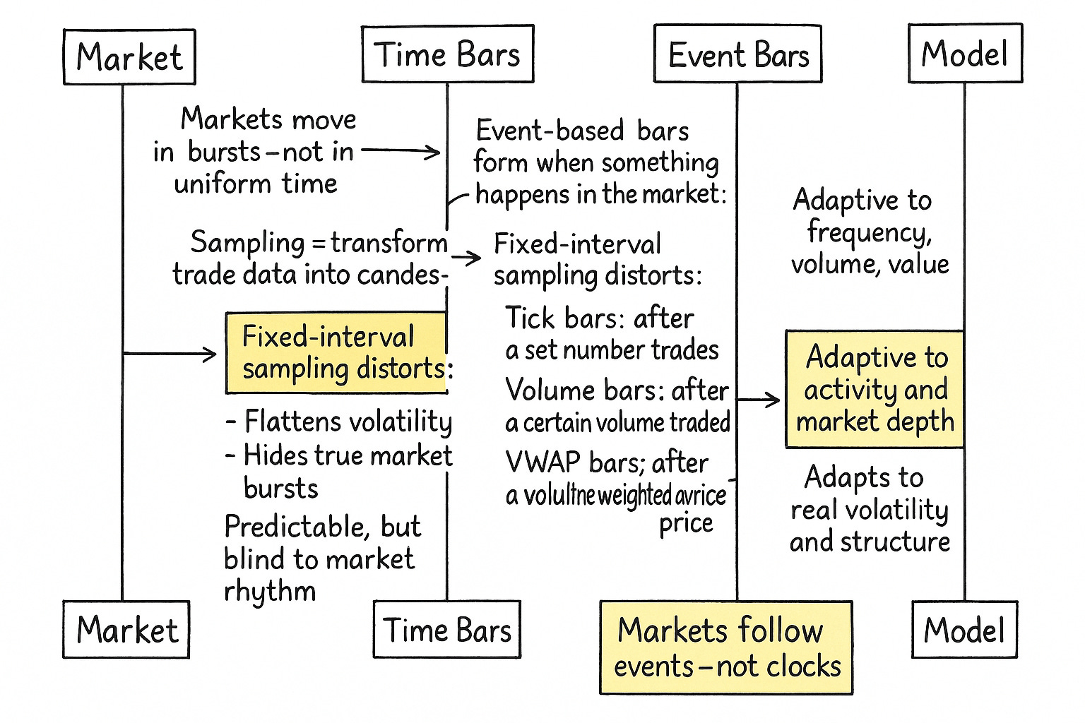
Standard time-based intervals often fail to capture meaningful changes in market behavior. Instead, choosing the right way to sample data—whether by volume, price change, or other criteria—becomes a crucial decision for building effective algorithmic strategies. Sampling isn’t just a technical detail; it shapes how well a strategy "sees" and responds to real market conditions.
The core idea is to consciously decide when and how to take snapshots of the market. Do we sample at fixed time intervals, like a security camera taking a picture every minute, regardless of activity? Or do we sample based on events, like a motion-activated camera that only records when something significant happens—a certain volume traded, a specific price movement, or a defined amount of dollar value exchanged? This decision is the first and perhaps most profound obstacle.
Market data, at their most granular level, generate events continuously. Every trade executed, every update to an order book, is a distinct piece of information. If we were to visualize this, it would be an unending, high-frequency stream of data points (ti, pi, vi), representing the time, price, and volume of each individual trade i.
Mathematically, let this stream of trades be denoted as:
where N can be astronomically large even for a single trading day.
The core of sampling is to define a sequence of "bar-closing" times, denoted {Tk} for k=1, 2, …, K. Once these Tk are determined by some rule, we aggregate the tick data within each interval (Tk-1, Tk] to form an Open-High-Low-Close bar, along with other relevant statistics like total volume, number of ticks, or total dollar value traded.
The fundamental aggregation formulas are:
openk=pfirst trade in interval (price of the first trade at or after Tk-1 if not using the previous close, or more commonly, the price of the first trade pik that starts the new bar).
highk=max{pi} for all trades i such that Tk-1<ti≤Tk.
lowk=min{pi} for all trades i such that Tk-1<ti≤Tk.
closek=plast trade in interval (price of the last trade pjk at or before Tk).
volumek=∑vi for all trades i within the interval.
ticksk=∑1 for all trades i within the interval.
dollar volumek = ∑(pi vi) for all trades i within the interval.
This presents an immediate contrast:
Continuous data: The raw, untamed flow of market events. Rich in detail, but overwhelming and computationally demanding. Like trying to drink directly from a waterfall.
Discrete data (aka bars): Structured snapshots derived from the continuous flow. Easier to analyze and model, but the act of discretization inherently involves information loss or distortion. Like scooping water with a cup–the cup's size and shape determine what you get.
And a primary choice:
Uniform (time-based) sampling: We observe the market at fixed time intervals, e.g., every minute, every hour. The rule for Tk is simply:
\(T_k = T_{k-1} + \Delta t.\)This is the “metronome” approach.
Event-driven sampling: We observe the market whenever a specific event threshold is met. This could be a certain number of ticks transacted, a certain volume traded, a specific price change—like Renko or Range bars—or a certain dollar value exchanged. The rule for Tk is more dynamic, triggered by market activity itself. This is the "seismograph" approach.
The misconception here is that one is inherently superior:
The reality is that the choice of sampling scheme is a lens that shapes our perception of market dynamics. A time-based bar might show low volatility during a period where many small trades occur, while a tick-based bar for the same period would show high activity. Neither is "wrong"; they are different perspectives on the same underlying reality. The initial obstacle is choosing which perspective aligns best with the phenomenon we're trying to model or the edge we're trying to exploit.
Mathematically, given a stream of trades (ti, pi, vi), we define a sequence of bar‐close times {Tk} via a rule, then aggregate:
and similarly volume, ticks, dollar volume.
Limitations of sampling bars
Sampling financial data into bars—such as time, tick, volume, or dollar bars—is a common practice in algorithmic trading and quantitative finance. It simplifies the analysis, modeling, and execution of trading strategies. However, this simplification comes with certain inherent limitations and risks that must be carefully managed:
Sampling inevitably reduces data granularity. All trades within a single bar are represented by only four prices: open, high, low, and close. Consequently, crucial intra-bar details, such as the precise sequence of trades, transient price spikes, and subtle order flow dynamics, are lost. This loss can obscure short-term market signals and reduce the responsiveness of certain trading strategies.
Different bar types inherently introduce sampling biases. Time bars, for instance, equally represent low and high activity periods, potentially underestimating bursts of market activity. Conversely, tick, volume, or dollar bars oversample active periods, distorting measures of average market behavior. Additionally, the irregular length of activity-based bars complicates the association of market data with external events such as news announcements or economic data releases.
The choice of bar size impacts volatility estimation. Too small a bar size may introduce microstructure noise, such as bid-ask bounce, inflating estimates of realized volatility. Conversely, too large a bar size smooths genuine price fluctuations, underestimating volatility. Moreover, irregular bar intervals require special adjustments when computing correlation and covariance, as standard estimators assume regularly spaced observations, potentially introducing additional bias.
Periodic market dynamics or cycles can be distorted through improper sampling, a phenomenon known as frequency aliasing. Incorrectly chosen bar sizes might misrepresent periodic behaviors as random fluctuations. Since the optimal bar length is not universally agreed upon and often empirically determined, there's a risk of overfitting strategies to historical data, undermining their robustness.
When sampling data independently across multiple assets, timing discrepancies arise. For instance, volume bars on two correlated assets will rarely align in time. This non-synchronization can introduce artificial lead-lag relationships, complicating cross-asset analysis and potentially resulting in spurious trading signals or misleading interpretations of market dynamics.

Time bars
Time-based bars are the most conventional and widely understood method of sampling. They are the grandfather clock of market analysis, steadily chiming out bars at predetermined intervals–seconds, minutes, hours, days.
For Time bars, the metric M(ti, pi, vi) is simply the elapsed time since the last tick,
However, it's more practically implemented by defining a fixed bar duration, Ltime. A new bar k starts at Tk-1. and closes at:
All ticks (ti, pi, vi) such that Tk-1<ti≤Tk are aggregated into bar k:
For the following implementations and in the posts to follow, I've used Hudson and Thames' implementation as a base. And although I created a different library, the tick, volume, dollar, and imbalance bars are based on their original idea.
Here the code idea:
class TimeBars(BaseBars):
    def __init__(self, units, res, batch_size=int(2e7)):
        super().__init__(None, batch_size)
        # Determine seconds per bar based on resolution ('D', 'H', 'MIN', 'S')
        secs = {'D': 86400, 'H': 3600, 'MIN': 60, 'S': 1}[res]
        self.threshold = units * secs  # Total seconds for the bar
        self.next_ts = None # Timestamp for the next bar close

    def _check_bar(self, t, p, bars):
        # Convert current trade timestamp to seconds
        ts = int(pd.to_datetime(t).timestamp())
        if self.next_ts is None:
            # Initialize the first bar's closing timestamp
            # It aligns to the next multiple of the threshold
            self.next_ts = ((ts // self.threshold) + 1) * self.threshold

        if ts >= self.next_ts:
            # Current trade's time is at or past the bar's closing time
            bars.append([
                pd.to_datetime(self.next_ts, unit='s'), # Bar closing time
                self.stats['cum_ticks'], self.open, self.high,
                self.low, self.close, self.stats['cum_vol'],
                self.stats['cum_buy_vol'], self.stats['cum_ticks'], # Redundant ticks?
                self.stats['cum_dollar']
            ])
            self.reset() # Reset accumulated stats for the new bar
            # Set the next closing time
            self.next_ts += self.threshold
This implementation defines a bar by a fixed duration (self.threshold in seconds). When a new trade arrives (_check_bar), its timestamp ts is compared to self.next_ts. If it's time to close the current bar, the aggregated OHLCV data is recorded, and self.next_ts is incremented by the bar duration. The BaseBars.reset() method clears out self.open, self.high, etc., for the next bar.
Advantages:
You get a fixed number of bars per day/week (e.g., 390 one-minute bars for a standard US equity trading day). This can simplify some modeling approaches.
Easy to understand, implement, and widely supported by charting platforms.
For very long-term analysis, time bars can offer a semblance of regularity, though this is often an illusion for financial returns.
Disadvantages:
Time bars form regardless of market activity. A 1-minute bar during a market freeze looks the same in duration as a 1-minute bar during a flash crash, yet they represent vastly different market states. This is like a reporter filing a story every hour, even if no news has happened for days, or too much news to fit in one report.
Periods of high activity—many trades, large volume—are crammed into the same time slot as periods of low activity. This can smooth out important volatility information or make it difficult to discern the true impact of rapid events.
Returns from time bars often exhibit heteroskedasticity—non-constant variance—and autocorrelation, precisely because market activity itself is clustered and not uniform over time. This complicates statistical modeling. For instance, volatility is typically high at market open and close, and lower mid-day. Time bars don't inherently adjust for this.
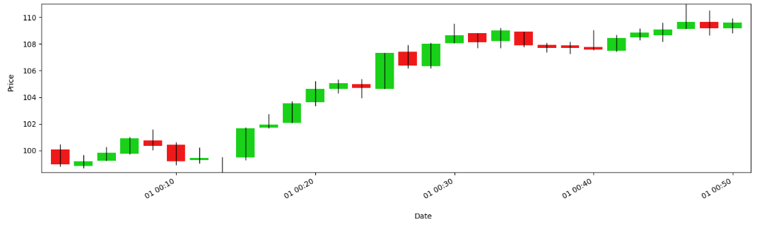
Let's visualize these types of bars. They're the classic bars, the ones offered by any charting platform:

This plot would typically show price movements over regularly spaced time intervals. The key takeaway is the uniformity of the x-axis intervals, regardless of how much or how little happened within them.
Tick bars
Tick bars offer a direct contrast to time bars. Instead of sampling based on the clock, they sample based on the number of transactions. A new bar is formed every time a predefined number of trades—ticks—has occurred. This is like measuring a journey not by hours passed, but by steps taken
For Tick bars, the metric M(ti, pi, vi)=1 (each trade is one unit). A bar k closes when the cumulative sum of these units within the bar,
reaches a predefined threshold Lticks—the number of ticks per bar. So, Sk≥Lticks.
The chunk of code in charge of that is:
class TickBars(BaseBars):
    def __init__(self, threshold, batch_size=int(2e7)):
        super().__init__('cum_ticks', batch_size) # metric is 'cum_ticks'
        self.threshold = threshold # Number of ticks per bar

    def _check_bar(self, t, p, bars):
        # 'limit' can be a fixed threshold or a dynamic one (e.g., pd.Series)
        limit = self.threshold.loc[t] if hasattr(self.threshold, 'loc') else self.threshold

        # self.stats['cum_ticks'] is incremented in BaseBars.run()
        if self.stats['cum_ticks'] >= limit:
            # Threshold reached, form a new bar
            bars.append([
                t, # Timestamp of the trade that completed the bar
                self.stats['cum_ticks'], # Actual ticks in bar (could be > threshold)
                self.open, self.high, self.low, self.close,
                self.stats['cum_vol'], self.stats['cum_buy_vol'],
                self.stats['cum_ticks'], # Actual ticks again
                self.stats['cum_dollar']
            ])
            self.reset() # Reset for the next bar
Here, self.threshold is the target number of ticks. self.stats['cum_ticks'] accumulates the count of trades. When this count hits the threshold, a bar is formed using the timestamp of the last trade that completed the bar.
Advantages:
Bars are formed more frequently during periods of high trading activity and less frequently during quiet periods. This naturally adapts to the market's pulse.
By sampling proportionally to activity, tick bars can sometimes lead to return distributions that are closer to Gaussian and exhibit less heteroskedasticity compared to time bars, as each bar encapsulates a similar amount of "market information" in terms of transaction count. This is a significant shift in perspective–we're seeking bars with uniform information content rather than uniform time duration.
Disadvantages:
The time duration of tick bars is not constant, making it harder to compare bar lengths or use models that assume fixed time steps. A 500-tick bar might span seconds during a frenzy or hours during a lull.
All ticks are treated equally, whether it's a 1-share trade or a 10,000-share block trade. A period of many tiny, insignificant trades could trigger more bars than a period with fewer, but much larger and more impactful, trades. This is a critical misconception to avoid: more ticks don't always mean more "significant" activity if trade sizes are small.
During extremely low activity periods—e.g., holidays, overnight for some assets—tick bars might take a very long time to form, leading to apparent data gaps if one is still thinking in calendar time.
Let’s visualize it:
This plot would show data points (bar closes) that are not evenly spaced in time. They would cluster during high-activity periods and spread out during low-activity ones. This visualization breaks the misconception that markets should be viewed through a fixed-time grid.
Volume bars & VWAP bars
While tick bars count transactions, volume bars aggregate trades until a specific total volume has been exchanged. This directly measures market participation in terms of share quantity. It's like waiting for a river to discharge a certain amount of water before taking a sample.
The metric is the volume of each trade, M(ti, pi, vi)=vi. A bar k closes when the cumulative volume,
reaches a predefined threshold Lvolume. So, Sk≥Lvolume.
We can model it by using:
class VolumeBars(BaseBars):
    def __init__(self, threshold, batch_size=int(2e7)):
        super().__init__('cum_vol', batch_size) # metric is 'cum_vol'
        self.threshold = threshold # Target volume per bar

    def _check_bar(self, t, p, bars):
        limit = self.threshold.loc[t] if hasattr(self.threshold, 'loc') else self.threshold
        # self.stats['cum_vol'] is incremented in BaseBars.run()
        if self.stats['cum_vol'] >= limit:
            bars.append([
                t, # Timestamp of the trade that completed the bar
                self.stats['cum_ticks'],
                self.open, self.high, self.low, self.close,
                self.stats['cum_vol'], # Actual volume in bar
                self.stats['cum_buy_vol'],
                self.stats['cum_ticks'],
                self.stats['cum_dollar']
            ])
            self.reset()
This structure is analogous to TickBars, but self.stats['cum_vol'] and self.threshold—for volume—are used.
VWAP bars or Volume-Weighted Average Price bars—are a variation. They close based on the same volume accumulation criterion as Volume Bars. However, their closing price is not the last trade price but the VWAP of all trades within that bar:
And the code snippet in charge is:
class VWAPBars(BaseBars):
    def __init__(self, volume_threshold, batch_size=int(2e7)):
        super().__init__(None, batch_size) # Metric for closing is volume based
        self.volume_threshold = volume_threshold

    def _check_bar(self, t, p, bars):
        if self.stats['cum_vol'] >= self.volume_threshold:
            # Calculate VWAP for the bar
            vwap = self.stats['cum_dollar'] / self.stats['cum_vol'] if self.stats['cum_vol'] > 0 else p
            bars.append([
                pd.to_datetime(t),
                self.stats['cum_ticks'],
                self.open, self.high, self.low, vwap, # VWAP is the close price
                self.stats['cum_vol'],
                self.stats['cum_buy_vol'],
                self.stats['cum_ticks'],
                self.stats['cum_dollar']
            ])
            self.reset()
The key difference is vwap = self.stats['cum_dollar'] / self.stats['cum_vol'] which becomes the closing price.
Advantages:
Each bar represents a similar amount of shares traded, which can be a better proxy for "information" or market impact than just time or number of trades.
VWAP bars can provide a more robust measure of the average price at which a certain volume was transacted, reducing noise from individual tick fluctuations.
Like tick bars, volume bars can lead to more well-behaved return distributions as they synchronize with market activity.
Disadvantages:
Similar to tick bars, the time duration of volume bars is not constant.
A single very large trade could complete a volume bar quickly. This might be desirable (as it reflects significant activity) or undesirable—if it distorts the bar's representativeness of typical flow.
The bar formation rule itself is based on volume, not how much the price moved while that volume was accumulating. A lot of volume could trade in a very tight price range, or a little volume could accompany a large price swing.
Let’s compare both, first volume bars and then VWAP bars:

This plot illustrates that each bar represents a roughly constant amount of volume traded, but the time taken to accumulate this volume varies, leading to non-uniform time spacing of the bars. The dual-axis helps visualize volume alongside price. This breaks the misconception that market time is solely calendar time; here, it's volume time.