


Table of contents:
Introduction.
Risk and limitations of adaptive bars.
Adaptive segementation and microstructural insights.
Delta bars.
EMA imbalance bars.
Quantile bars.
Run bars.
Which bar should I choose?
Before you begin, remember that you have an index with the newsletter content organized by clicking on “Read full story” in this image.

Introduction
Previous discussions systematically highlighted the limitations inherent in time-based aggregation methods: heteroskedastic returns, distorted volatility signatures, and embedded structural biases. Event-driven alternatives—tick, volume, and dollar bars—were introduced to address these issues by sampling according to market activity rather than fixed chronological intervals. However, implementing these adaptive methods presents non-trivial optimization challenges requiring rigorous quantitative analysis.
While activity-based bars significantly improve certain statistical characteristics, such as achieving closer-to-normalized return distributions and reducing serial correlation, each type carries context-specific drawbacks:
Regime sensitivity:
Volume bars presuppose uniform informational density per traded unit. During low-volatility periods—e.g., when VIX < 12—a 10,000-share bar might span 15 minutes or more, blending multiple equilibrium states into a single bar.
Dollar bars standardize by notional value, yet can amplify exposure to tail events. A $2 million bar for SPY during a 5σ volatility spike—such as a major FOMC announcement—might encapsulate nearly the entire day's return variance.
Microstructural artifacts:
Tick bars disregard trade size variability. In equity markets, a 1,000-tick bar might aggregate:
1,000 small, retail-sized trades—e.g., 0.1 lots each—dominated by noise.
A single institutional iceberg order, dominated by significant market signals.
This variability breaches the implicit assumption of ergodicity inherent in tick-based sampling.
Temporal misalignment:
Irregular bar intervals complicate:
Non-synchronous bar closes across different assets create challenges in aligning data.
Variable computational latency per bar can affect the timeliness of actionable signals.
Temporal inconsistencies might blur the precise impact of market catalysts.
Building upon the foundational understanding of market data representation established previously, we now face the critical challenge of operationalizing adaptive, event-driven sampling without introducing fresh biases or excessive computational burdens. The transition from time-based to event-driven bars solves previous aggregation issues but simultaneously uncovers new microstructural complexities.
Adaptive or imbalance-driven bars notably enhance statistical properties, including normalized return distributions and reduced serial correlation. Despite these improvements, each method carries specific considerations:
Delta bars track signed trade imbalances, forming a bar when cumulative imbalance exceeds a specified threshold. While they effectively capture shifts in buyer-seller dynamics, precise threshold selection remains crucial.
EMA imbalance bars dynamically adjust tick thresholds based on an exponentially weighted moving average of recent imbalances. This method helps respond adaptively to changing market conditions but requires careful tuning of the EWMA parameters.
Quantile bars maintain a historical window of recent bar sizes, setting thresholds based on specified quantiles. This approach dynamically adjusts to market volatility, capturing significant market moves more reliably than static thresholds.
Run bars focus on sequences of trades with consistent directional signs, forming bars when the run exceeds a defined length. This captures sustained directional momentum, though the choice of run length significantly impacts sensitivity.
Consider breakout detection scenarios: adaptive bars resolve intra-bar volatility concerns but can introduce vulnerabilities if improperly parameterized. For example, Delta bars set with overly sensitive thresholds may capture too many false signals, whereas overly rigid Run bars might miss critical momentum shifts. These practical trade-offs directly affect alpha decay and strategy reliability.
Effectively navigating these complexities involves three pivotal strategies:
Multi-dimensional sampling: Integrating dynamic thresholds or combining indicators, such as blending EMA-based methods with quantile-driven approaches, to form more context-sensitive bars.
Strategy-aware calibration: Aligning bar parameters explicitly with the alpha capture horizons of specific strategies, distinguishing clearly between short-term and longer-term trading approaches.
Dynamic validation: Continuously assessing bar stability and responsiveness through statistical validation methods, ensuring adaptive bars reliably capture genuine market conditions.
Implementing these adaptive sampling strategies requires meticulous quantitative analysis and practical adjustments. Traders must continually balance accuracy with computational efficiency, refining adaptive frameworks to reflect evolving market dynamics through iterative feedback loops.
Ultimately, successfully employing adaptive bars transcends data enhancement; it fundamentally seeks to improve trading model precision and reliability. Allowing market-driven signals to directly inform strategic decisions is crucial for sustained performance and resilience in algorithmic trading.
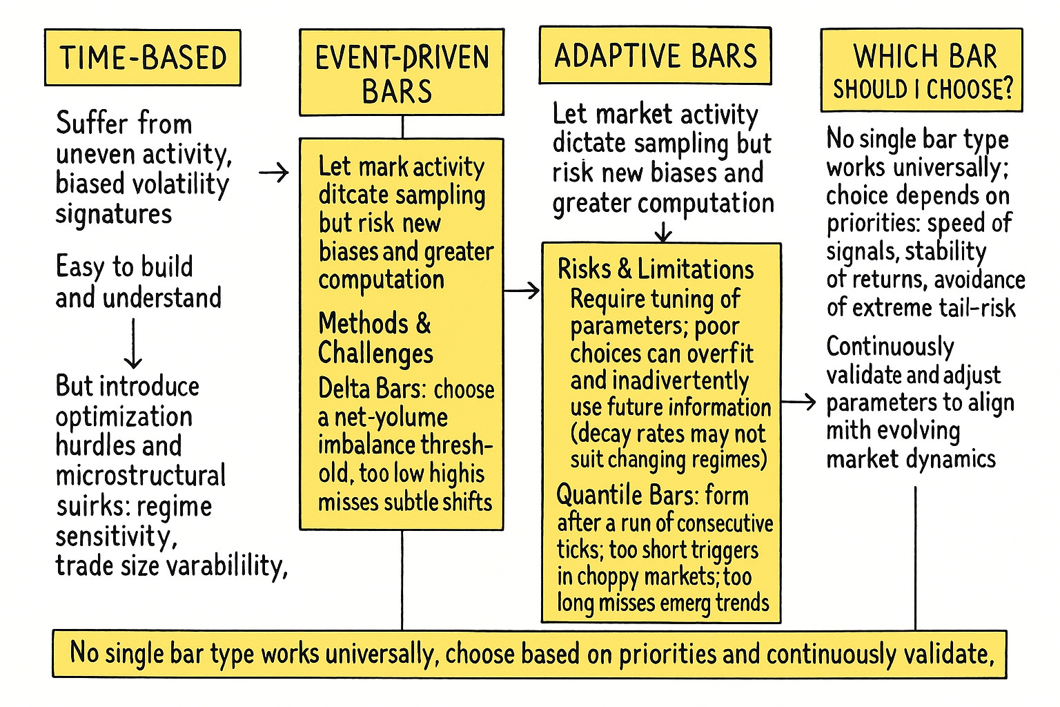
Risk and limitations of adaptive bars
Imagine you're trying to understand crowd behavior. Would you take a photo every five minutes regardless of what's happening? Or would you take a photo every time, say, a hundred people gather in one spot, or when the noise level reaches a certain peak? The latter approach, event-driven and adaptive, is far more likely to capture significant moments. This is precisely the philosophy behind information-driven bars in algorithmic trading. We're aiming to create data segments that are more homogeneous in terms of the information they contain, leading to more statistically well-behaved series and, hopefully, more potent trading signals. It’s a move from a dumb, fixed-window approach to an intelligent, data-sensitive one.
However, it's no walk in the park. This path is riddled with general pitfalls that demand careful attention:
Adaptive bars often come with their own set of parameters—e.g., imbalance thresholds, window sizes for moving averages, quantile levels. Choosing these parameters appropriately is critical. There's a significant risk of overfitting to historical data.
While the goal is to create bars that are more homogeneous in information content—e.g., each bar represents a similar amount of volume or imbalance—this can sometimes lead to bars that vary wildly in their time duration.
One must be careful in defining current bar size or current path to ensure no information from future ticks—relative to the bar's conceptual closing tick—inadvertently influences the decision to close the current bar, especially in backtesting.
Besides, the central challenge remains defining meaningful market activity across these methods:
Delta bars clearly indicate shifts in trade dominance but depend heavily on threshold accuracy.
EMA imbalance bars provide adaptive responsiveness yet require continuous recalibration to maintain effectiveness.
Quantile bars robustly reflect current volatility regimes, yet historical window length can influence responsiveness.
Run bars effectively highlight directional continuity but need careful parameter tuning to avoid oversensitivity or lag.

Adaptive segementation and microstructural insights
Having established the why and the inherent complexities, let's delve into the how. We will now explore different adaptive bar construction. Each offers a unique lens to face the market.
But before we dissect specific bar types, let's cement the foundational principle:
Adaptive bars strive to synchronize with the intrinsic rhythm of the market, not an extrinsic clock. The core idea is to sample observations when a sufficient amount of information has accumulated. This information can be defined in various ways–volume, dollar value traded, number of ticks, price volatility, order flow imbalance, or even more abstract mathematical properties of the price path.
Contrast this with time bars. If we have a 1-minute bar chart, each bar represents 60 seconds of price action, regardless of whether 100 trades or 10,000 trades occurred. An adaptive bar, say a volume bar set to 1,000 shares, will only complete once 1,000 shares have traded. This could take 5 seconds during a frenzy or 15 minutes during a lull.
The beauty of this approach lies in its ability to produce a data series where each bar, by construction, represents a similar market activity. This often leads to statistical properties that are more desirable for modeling:
Volatility tends to be more stable across bars.
Bar returns are often closer to a normal distribution, which simplifies many statistical models.
By filtering out periods of low activity—which are essentially noise from an information perspective—these bars can sharpen the signals.
This fundamental shift—from time-based sampling to information-based sampling—is the gateway to a more nuanced and potentially more profitable understanding of market dynamics. It’s about letting the market dictate the pace of our analysis.
Now, let's get specific. One of the most intuitive ways to capture buying and selling pressure is to look at order imbalance. DeltaBars do precisely this, focusing on the net signed volume.
The core idea is to track the cumulative difference between buyer-initiated volume and seller-initiated volume—or a proxy for it. We define the delta for each tick. A common way to define the signed volume vi for a tick i is: if the tick resulted from a buyer crossing the spread, it's +vi; if it's a seller crossing the spread, it's −vi. More simply, as in the provided information, we can look at the change in value based on the tick direction:
Let vi be the volume or dollar value of tick i. The signed imbalance Δi for that tick can be defined as:
Alternatively, a formulation like Δi=2×1{buy tick}vi−vi aims to capture this, where 1{buy tick} is an indicator function that is 1 if the tick is classified as a buy and 0 otherwise. This effectively results in +vi for a buy and −vi for a sell—assuming vi is always positive.
A DeltaBar is formed when the absolute value of the cumulative signed imbalance since the last bar formation exceeds a predefined threshold Δ0:
where N is the number of ticks in the current, forming bar.
Let’s implement this type of bars: