

[WITH CODE] Feature selection: Wrapper-based feature selection methods
Model-dependent approaches
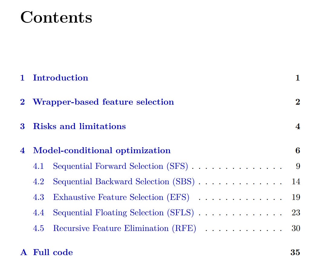
Table of contents:
Introduction.
Wrapper-based feature selection.
Risks and limitations.
Model-conditional optimization.
Sequential Forward Selection (SFS).
Sequential Backward Selection (SBS).
Exhaustive Feature Selection (EFS).
Sequential Floating Selection (SFLS)
Recursive Feature Elimination (RFE).
Audio Note: Before we begin, remember that if you’re accessing this article through the Substack app, you can listen to it instead of reading it.
Before you begin, remember that you have an index with the newsletter content organized by clicking on the image below.
Introduction
Feature selection is often presented as a simple cleanup step… remove the weak variables, keep the useful ones, and move on. In practice, it is much closer to a research decision about what information the model is allowed to trust.
Every feature added to a trading system creates a cost. It may require another data source, increase latency, make the model harder to interpret, or create another opportunity for overfitting.
Wrapper-based methods approach this problem from a practical perspective. Instead of judging features in isolation, they test them through the model that will actually use them. This makes the selection process more realistic, because a feature only matters when it improves the behaviour of the complete model under a credible validation framework.
You can go deeper in warpper methods by checking this two papers:
Each method follows a different search philosophy, from gradually building a compact feature set to pruning a large one or evaluating every feasible combination. The goal is to understand how each method deals with the trade-off between predictive value, stability, and model complexity. By comparing them under the same structure, it becomes easier to see when a method is useful, where it can fail, and how its selection path affects the final trading model.
Wrapper-based feature selection
Identifying a reliable predictive signal requires more than measuring isolated statistical correlations. Wrapper-based feature selection provides a methodology to evaluate the predictive power of specific feature combinations. This approach integrates the target model into the selection loop. The system wraps a search algorithm around the predictive model and uses empirical validation performance to score candidate feature subsets.
To understand the architecture of wrapper methods, we must examine other selection paradigms:
Filter methods operate outside the boundaries of any model. They evaluate features based on intrinsic statistical properties, such as variance or mutual information with the target variable. This standalone structure gives filter methods a lightweight computational profile. They isolate fundamental data characteristics and separate the data from the final algorithmic interpretation. This separation forces filter methods to overlook complex feature interactions.
Wrapper methods take a distinct path. They evaluate features by training and validating a defined model in repeated cycles. The wrapper treats the target algorithm as a direct scoring engine. It tests candidate subsets of features and measures their impact on out-of-sample performance. This approach requires retraining the model from a blank state for every candidate subset evaluated, which creates an immense computational cost. Because these methods remain model-dependent, they offer an honest measurement of predictive utility in live trading scenarios.
Embedded methods incorporate feature selection into the model training process. Algorithms like Lasso regression penalize lower-impact features during the construction of their mathematical structure. This mechanism merges selection and training into a single phase, which generates a moderate computational cost. The selection process remains locked to the internal mechanics of that chosen algorithm.
A complete wrapper architecture relies on four fundamental components that operate in a continuous loop:
The search space establishes the boundaries of all available candidate features.
The search strategy dictates the algorithmic trajectory to navigate the combinations.
The evaluation metric provides the quantitative objective function to measure model predictions.
The underlying model defines the algorithm that maps candidate inputs to the target variable.
Wrappers evaluate features in collective groups. This structure gives them the capability to identify joint signal interactions that single-variable statistical filters exclude. For example, order flow dynamics and volatility regimes interact in nuanced patterns and the wrapper asks a specific question “Does the inclusion of this feature improve the predictive accuracy of this specific model?” This collective evaluation makes wrappers suited for discovering market dynamics. The use of the model as a direct scoring engine ties the value of a feature to the tested environment, something that shapes the optimization required for live trading.
Risks and limitations
This sounds trivial from a standard machine learning perspective.
“Choose a model, choose a feature subset, train the model, evaluate the score, and repeat. The method transforms feature selection into a clean optimization problem.”
However, in trading, that statement hides a difficult engineering problem because the score itself is unstable, labels contain noise, observations are serially dependent, etc. As a result, a feature subset that looks like pure gold during one sample can become a major source of loses the second market volatility spikes or participant behavior shifts.
The trouble with financial models starts at the foundation with a messy problem called temporal contamination. Standard cross-validation requires independent data points, but market data streams possess a strict order, a clear dependency, and a constant overlap. Breaking this data into random folds causes leakage, because future price action bleeds into past training sets. Fixing this error requires a boundary, which is where purging and embargoing come into play to isolate the training data from the test data.
Once that data leak is under control, a different headache appears, known as the curse of multiple testing. Wrapper algorithms sift through piles of potential features, a process that inflates the top score by pure chance. A huge search space guarantees a spectacular winner born from total noise. Without a strict separation of time horizons during validation, the algorithm flags a historical fluke instead of a true lasting edge.
These flawed features cause more damage due to model dependence, meaning a feature set has zero portability across different setups. A group of features built for a linear model falls apart inside a decision tree. Features picked via Ridge regression turn useless under Lasso regularization. Binary classifier inputs lose their grip when converted into continuous position sizing logic. The whole selection process builds a house of cards that links the model class, the features, the labels, and the validation into one single knot. A change to one thread collapses the entire framework.
And what about research drift? It acts as a hidden form of data snooping. Running a loop through forward selection, backward selection, and recursive elimination stacks up the hidden trial count. Tweaking the metrics, shifting the data splits, or altering the label horizons to chase better historical returns introduces a selection bias. This game ruins the validity of standard significance tests.
Model-conditional optimization
At its core, a wrapper method selects features by treating the underlying model as a black box and evaluating performance across various candidate subsets. Because the feature set is judged through the lens of a specific model and metric, context dictates everything. The exact same feature can prove useful under one model architecture while remaining useless under another.
To formalize this process, let the full candidate feature pool be defined as F={f1,f2,…,fp}. From this pool, any given candidate subset is represented as S⊆F.
Now, assuming a specific model class M, a training dataset Dtrain, a validation dataset Dval, and a scoring function J, the wrapper selection process solves the following optimization problem:
Where the fitted model relies entirely on the chosen feature subset:
The path taken to find S* depends on how you define the search space boundaries. An exhaustive feature selection routine evaluates every single possible subset in the space. Conversely, sequential methods restrict the computational burden by following a rigid, step-by-step path. Meanwhile, recursive feature elimination leverages the model’s internal feature rankings to determine the deletion order.
The objective function J requires far more scrutiny than the search algorithm itself. It is easy for a wrapper to optimize a clean statistical metric and lose money. For instance, a model boasting a high Information Coefficient can deliver negative realized returns if the signal exhibits weak ranking power near the critical threshold used for execution. Furthermore, a model with flawless gross performance fails the moment you incorporate exchange fees, slippage, or borrow costs.
To force the wrapper to respect these execution boundaries, the objective function requires a penalty structure:
In this functional, rt(S) represents the strategy returns generated by the model using feature subset S. The penalty terms translate market fees into the optimization. C(S) captures execution friction and turnover costs, while Ω(S) imposes a penalty on the dimension of the subset. A subset that marginally improves predictive power at the expense of skyrocketing turnover will degrade the net equity curve. Likewise, a subset that performs perfectly in one data fold but collapses in another introduces unstable deployment behavior.
This is why researchers focus less on the final feature list and look instead at the structural stability of the selection process. The result must satisfy several clear operational conditions:
The selected subset appears persistently across distinct temporal folds.
The chosen features survive aggressive changes to the underlying scoring metric.
The subset keeps strategy turnover within the fund’s execution capacity.
The selected features reduce live decision complexity.
The subset improves net performance after accounting for all fees and costs.
The features demonstrate a plausible connection to known market microstructure mechanics.
The model performance degrades slowly when the market regime shifts.
This brings us to a misconception. The idea that wrapper methods discover an objectively “best” set of features. In reality, they find the optimal subset constrained by a specific search path, a chosen model class, a single metric, a finite sample size, and a defined validation protocol.
Visualizing this behavior clarifies why simpler selection methods fail.
Viewed independently, both x1 and x2 demonstrate a flat, weak relationship hovering around zero. Together, however, they may define a significant structural edge. This interaction highlights the exact reason why univariate filters fail to identify effective trading combinations.
To translate this into a concrete trading scenario, suppose x1 represents short-term price reversal pressure, while x2 represents prevailing bid-ask liquidity conditions. Reversal strategies often perform well during specific liquidity regimes but fail during others. A univariate filter evaluating x1 in isolation would reject the feature due to its poor average performance. A wrapper method retains it because the underlying model evaluates the conditional interaction between the two variables.
Sequential Forward Selection (SFS)
SFS begins with an empty feature set and adds exactly one feature at a time. At each step, the algorithm chooses the candidate that delivers the largest immediate mathematical improvement in the target objective function.
Let the current selected set at step k be denoted as Sk. The algorithm chooses the optimal addition
Then it updates the state space
The algorithm terminates when the score improvement falls below a defined threshold, when a hard target subset size is reached, or when the validation performance begins to show signs of deterioration.
SFS is attractive because it guarantees compact models. Compact models possess immense engineering value. A low-latency execution model with five stable features has operational advantages over a bloated model with fifty fragile inputs. Fewer features reduce data pipeline dependencies, time-synchronization errors, memory footprint, and total inference latency. In execution environments where any individual data feed can drop or delay, a smaller feature set provides a definitive robustness advantage.
Imagine an intraday market-making model evaluating the spread, the trade size, the order book imbalance, the short-term realized volatility, and the last price displacement. Forward selection builds a minimal subset capturing the vast majority of the useful effect while avoiding slow or noisy features.
Forward selection provides another benefit in high-dimensional settings. It starts from zero features, ensuring the early model fits remain numerically stable. Backward procedures begin with the full matrix. The full matrix becomes ill-conditioned when p is large, features exhibit collinearity, or the temporal sample size is constrained. But in this case it avoids the initial full-dimensional matrix inversion problem inherent in linear models.
The primary limitation involves severe path dependence. The algorithm is greedy. It selects the best immediate addition and carries that rigid choice forward forever. A feature that looks weak early could become useful later when paired with another specific feature. Forward selection misses that pair because neither feature produces enough standalone improvement at the very beginning of the search path.
A trading-safe forward step evaluates candidates on temporal validation blocks
The model is trained on a training segment that excludes the validation segment and its required embargo neighborhood. The score averages across the folds and is more credible than a feature selected on a single randomized validation slice.
Many implementations stop at an arbitrary fixed number of features. But in our context, the subset size must be a direct consequence of measured marginal utility versus cost. Let the marginal gain be
A termination rule requires Δk>τ where τ includes a “premium”. That premium scales higher when a feature is computationally slow, or statistically unstable
Other rules use a penalized objective
where |S| penalizes dimensionality and Cops penalizes specific costly inputs.
Forward selection provides a diagnostic output for the researcher. The marginal contribution curve maps the precise geometry of the alpha extraction process. Plotting the sequential step-by-step score creates a direct visual representation of diminishing returns. If the first three features add the vast majority of the predictive value and the next five add microscopic improvements, the model has reached its absolute maximum useful complexity.
This type of system relies on a core directional driver, like a distinct volatility adjustment, and a liquidity filter. Evaluating further correlated technical variations adds zero edge. Forcing the model past this structural plateau increases execution latency and guarantees parameter overfitting in production. Furthermore, if the out-of-sample score keeps rising across dozens of consecutive feature additions, the researcher must investigate the foundational data pipeline.
On the other hand, an upward curve that never flattens proves that severe validation leakage or unchecked selection bias is artificially driving the continuous improvement. The algorithm is memorizing the specific validation sequence through overlapping return horizons, un-lagged data releases, or future price contamination.
Let’s implement it:
def sequential_forward_selection(
X,
y,
splits,
max_features=None,
min_improvement=0.0,
alpha=1.0,
metric="neg_mse",
complexity_penalty=0.0,
feature_costs=None,
candidate_features=None,
):
"""
Start with an empty feature set and greedily add the best feature.
The algorithm stops when:
- max_features is reached
- no candidates remain
- the best marginal improvement is below min_improvement
"""
X, y = _validate_xy(X, y)
candidates = _candidate_pool(X.shape[1], candidate_features)
if max_features is None:
max_features = candidates.size
max_features = min(int(max_features), candidates.size)
selected = []
remaining = candidates.tolist()
current_score = evaluate_subset(
X=X,
y=y,
feature_indices=selected,
splits=splits,
alpha=alpha,
metric=metric,
complexity_penalty=complexity_penalty,
feature_costs=feature_costs,
)
history = []
while remaining and len(selected) < max_features:
best_feature = None
best_score = -np.inf
for feature in remaining:
candidate_subset = selected + [feature]
score = evaluate_subset(
X=X,
y=y,
feature_indices=candidate_subset,
splits=splits,
alpha=alpha,
metric=metric,
complexity_penalty=complexity_penalty,
feature_costs=feature_costs,
)
if score > best_score:
best_score = score
best_feature = feature
improvement = best_score - current_score
if improvement <= float(min_improvement):
break
selected.append(best_feature)
remaining.remove(best_feature)
current_score = best_score
history.append(
{
"step": len(history) + 1,
"action": "add",
"feature": int(best_feature),
"score": float(current_score),
"improvement": float(improvement),
"subset": tuple(selected),
}
)
return np.asarray(selected, dtype=np.int64), historyThe marginal-gain profile requires intense review across folds. A feature that appears in one single fold is less credible than a feature repeatedly selected across multiple market regimes.
SFS excels under specific trading conditions:
The candidate feature pool is big.
The desired model is compact.
Feature interactions are moderate rather than complex.
The objective functional penalizes costs and turnover.
The training procedure uses purged temporal validation.
The research protocol fixes the search budget before execution.
The selected path remains stable across time.
The interpretation remains straightforward. Forward selection fails to be a universal feature discovery engine. It represents a strict incremental capital allocation procedure. Each feature receives allocation inside the model exclusively when it proves validated marginal utility. The final selected subset functions as a sparse, highly robust decision layer.
Sequential Backward Selection (SBS)
SBS begins with the complete, full-dimensional feature set and removes one feature at a time. At each specific step, the algorithm discards the feature whose removal causes the absolute smallest loss in target performance.
Let the current feature set at step k be denoted as Sk. The algorithm chooses the optimal removal candidate
Then it updates the state space by shrinking it
It looks pretty similar than the previous one, right? But it represents a different mathematical philosophy. Forward selection asks which feature earns the right to enter. Backward selection asks which feature deserves immediate eviction. That inversion is interesting when features possess joint predictive value.
Market data is saturated with features that could generate alpha—or smart beta— through interaction. Consider a small-cap mean-reversion signal where the overnight gap size matters when the opening liquidity exceeds a specific threshold. Forward selection misses these structures because each individual component looks statistically meaningless alone. Backward selection starts with the complete interaction structure intact and prunes away the dead weight.
The primary advantage of backward selection is its respect for joint information geometry at the start of the process. The disadvantage involves computational cost and severe numerical fragility. Early backward steps require fitting complex models containing almost every single candidate feature. When the feature matrix is wide, collinear, and saturated with noise, those initial model fits become unstable.
A full feature matrix in trading usually contains dozens of redundant transformations of the exact same underlying price path. The matrix contains returns over several horizons, various volatility estimators, moving average distance metrics, breakout flags, range ratios, candlestick wick metrics, and a pretty long list. These variables create a poorly conditioned design matrix.
For a linear model utilizing design matrix XS, the condition number κ determines the stability of the solution
When features are collinear, the minimum eigenvalue approaches zero, and κ explodes. A condition number means microscopic data perturbations produce coefficient changes. Backward selection ranks features terribly when the fitted model possesses this level of instability.
This approach requires feature clustering or Ridge regularization prior to initiating the backward pass. The goal is to extract redundancy from a verified joint signal structure. The scoring function guiding the backward removal must be calculated net of all frictional costs. Backward selection retains features that improve gross accuracy while increasing turnover if the score ignores that turnover. And here is the issue, the model looks good statistically but fails economically.
Let’s see how this look from coding perspective:
def sequential_backward_selection(
X,
y,
splits,
target_features=1,
max_score_loss=None,
alpha=1.0,
metric="neg_mse",
complexity_penalty=0.0,
feature_costs=None,
candidate_features=None,
):
"""
Start with the complete feature set and remove one feature at a time.
At each iteration, remove the feature whose exclusion produces the
highest validation score.
"""
X, y = _validate_xy(X, y)
candidates = _candidate_pool(X.shape[1], candidate_features)
target_features = int(target_features)
if target_features < 1 or target_features > candidates.size:
raise ValueError(
"target_features must be between 1 and the candidate pool size."
)
selected = candidates.tolist()
current_score = evaluate_subset(
X=X,
y=y,
feature_indices=selected,
splits=splits,
alpha=alpha,
metric=metric,
complexity_penalty=complexity_penalty,
feature_costs=feature_costs,
)
history = []
while len(selected) > target_features:
best_removed_feature = None
best_subset = None
best_score = -np.inf
for feature in selected:
candidate_subset = [
selected_feature
for selected_feature in selected
if selected_feature != feature
]
score = evaluate_subset(
X=X,
y=y,
feature_indices=candidate_subset,
splits=splits,
alpha=alpha,
metric=metric,
complexity_penalty=complexity_penalty,
feature_costs=feature_costs,
)
if score > best_score:
best_score = score
best_removed_feature = feature
best_subset = candidate_subset
score_loss = current_score - best_score
if (
max_score_loss is not None
and score_loss > float(max_score_loss)
):
break
selected = best_subset
current_score = best_score
history.append(
{
"step": len(history) + 1,
"action": "remove",
"feature": int(best_removed_feature),
"score": float(current_score),
"score_loss": float(score_loss),
"subset": tuple(selected),
}
)
return np.asarray(selected, dtype=np.int64), historyThe backward perspective proves valuable when the researcher suspects redundancy. Suppose the candidate matrix contains the 5-minute return, the 15-minute return, the 30-minute return, the 1-hour return, the distance to daily VWAP, the realized volatility, the ATR ratio, the spread percentile, and the opening range position. Several of these variables overlap geometrically. The model leverages them as correlated versions of the exact same latent state. Backward selection identifies and removes features whose absence changes the predictive distribution. The final result is a streamlined representation of an initial state space.
The defining statistic here is the conditional performance loss
The microscopic value for L(f | S) proves the feature contributes nothing after accounting for the presence of all other features. This implies the feature adds zero conditional value to the current set. It is redundant.
“Backward selection plays a role in post-research simplification. A quantitative researcher begins with a broad, complex model, utilizes backward selection to prune all redundant inputs, and then retrains the model from scratch on the radically reduced set. The final model boasts lower operational complexity, execution speed, and improved interpretability.”
Backward selection also demands safeguards:
The full feature model requires enforced numerical stability through regularization.
The validation protocol requires purged temporal blocking.
The entire removal path requires evaluation across multiple folds.
The final subset requires total retraining from a blank state.
The selected subset requires testing on untouched holdout data.
The pruning decision requires metrics based entirely on net trading performance.
A useful diagnostic is the removal curve, where if removing features barely alters the net performance for twenty consecutive steps, the original feature set contained redundancy. If the net performance collapses instantly after removing one specific feature, that feature represents a structural pillar of the model. And if performance actually improves as features are removed, the original set was saturated with noise.
Exhaustive Feature Selection (EFS)
EFS evaluates every possible subset of the candidate feature set. If the environment contains p features, the number of non-empty subsets is governed by the relation
This combinatorial explosion grows with terrifying speed. With 10 features, the engine tests 1,023 subsets. With 20 features, the engine tests 1,048,575 subsets. With 30 features, the engine tests 1,073,741,823 subsets. With 40 features, the engine evaluates more than one trillion distinct subsets.
Exhaustive search guarantees finding the absolute “best” subset within the defined search space. Greedy methods frequently miss the global optimum because of the restricted trajectory. Exhaustive search evaluates all paths simultaneously. For small feature sets, this capability is pretty valuable.
Every single subset requires training, validation, and scoring. If the model requires recalibration across rolling windows, the total computational cost multiplies by the number of windows. If the strategy spans multiple assets, the total cost multiplies again. If the score utilizes purged cross-validation, the cost multiplies by the total number of folds.
A simplified cost expression defines the boundary
where K is the validation folds, W is the rolling windows, A is the asset count, and Cfit is the hardware time required to fit one model.
For low latency infrastructure, this cost becomes something impossible. This kind of models require continuous recalibration, with micro or even nanosecond latency budgets. Exhaustive search across a large feature matrix conflicts with that operating environment.
On the other hand, choosing three factors—tiny feature set—from a universe of eight candidates is a reasonable exhaustive problem. Selecting a compact portfolio allocation model from a small universe of carry, value, momentum, inflation, liquidity, and growth factors justifies exhaustive evaluation. Here the researcher runs the exhaustive engine and compares the results of forward, backward, and floating methods against the known exhaustive optimum. If the greedy methods lock onto near-optimal subsets at a fraction of the computational cost, the greedy methods become verified production tools.
The researcher reduces the search space by enforcing subset size caps. Define the bounded space as
The number of evaluated subsets collapses to
For p = 40 and q = 3, the engine evaluates a manageable 10.700 subsets. Full exhaustive search over 40 features is nonsense. There is another issue here, this kind of search exponentially increases overfitting risk because it tests an astronomical number of alternatives. The more subsets tested, the higher the expected maximum score under pure noise.
The simulation generates pure Gaussian noise scores for thousands of subsets. The mean score of the population remains firmly anchored at zero. The selected maximum score rises as the number of tested subsets grows. The selected winner looks impressive despite every single candidate possessing zero true statistical edge.
Let Z1, Z2, …, ZM be validation scores for M candidate subsets under a null setting where each score is independent standard normal noise. The selected maximum score is
Even though E[Zi] = 0, extreme value theory proves that the expected value of the maximum grows proportionally to √(ln M). The larger M becomes, the larger the expected illusion of edge becomes.
This represents the defining danger of exhaustive search. The selected subset from an exhaustive search operates as a hypothesis generated by a machine. It identifies the best subset in-sample. The best in-sample subset frequently represents the absolute best historical accident. Due to that, this approach needs nested validation protocols and synthetic data validation for independent verification.
Let’s see how to implement it:
def exhaustive_feature_selection(
X,
y,
splits,
min_features=1,
max_features=None,
max_evaluations=100_000,
alpha=1.0,
metric="neg_mse",
complexity_penalty=0.0,
feature_costs=None,
candidate_features=None,
):
"""
Evaluate every possible subset inside the requested size range.
A safety limit prevents accidental combinatorial explosions.
"""
X, y = _validate_xy(X, y)
candidates = _candidate_pool(X.shape[1], candidate_features)
number_of_candidates = candidates.size
min_features = int(min_features)
if max_features is None:
max_features = number_of_candidates
max_features = int(max_features)
if min_features < 1:
raise ValueError("min_features must be at least 1.")
if (
max_features < min_features
or max_features > number_of_candidates
):
raise ValueError(
"max_features must be between min_features and the pool size."
)
best_subset = None
best_score = -np.inf
evaluations = 0
history = []
for mask in range(1, 1 << number_of_candidates):
subset_size = mask.bit_count()
if subset_size < min_features:
continue
if subset_size > max_features:
continue
evaluations += 1
if evaluations > int(max_evaluations):
raise RuntimeError(
"The exhaustive search exceeded max_evaluations. "
"Reduce the candidate pool or max_features."
)
local_positions = [
position
for position in range(number_of_candidates)
if (mask >> position) & 1
]
candidate_subset = candidates[local_positions].tolist()
score = evaluate_subset(
X=X,
y=y,
feature_indices=candidate_subset,
splits=splits,
alpha=alpha,
metric=metric,
complexity_penalty=complexity_penalty,
feature_costs=feature_costs,
)
if score > best_score:
best_score = score
best_subset = candidate_subset
history.append(
{
"evaluation": evaluations,
"score": float(best_score),
"subset": tuple(best_subset),
}
)
return np.asarray(best_subset, dtype=np.int64), historySequential Floating Selection (SFLS)
SFLS extends standard forward selection by integrating a backtracking mechanism. Standard forward selection adds a feature and keeps it permanently locked inside the model. Floating selection adds a feature, then checks whether removing one of the previously selected features improves the subset performance. The selected set expands and contracts during the search trajectory.
The forward addition step evaluates the marginal improvement
After officially adding f*, the backward correction step initiates a brutal internal audit. It searches for any weak link inside the newly expanded set
This formulation instructs the algorithm to temporarily exclude every single feature residing in the model, one at a time. It measures the exact performance degradation or improvement caused by that specific exclusion. The term Sk+1\{g} represents the state of the model acting without the candidate feature g. This internal check applies equally to the newest addition and to the very first feature selected at the beginning of the search path.
If removing g* improves the objective score over the previous historical maximum, the algorithm removes it, losing its allocation. The logic here relies on the shifting marginal utility of information. A feature providing immense value at step two becomes obsolete at step seven because the newly added features map the exact same latent market state with better precision.
This structural mechanism creates a self-correcting path through the subset space. The selected set expands and contracts dynamically. The algorithm regains degrees of freedom by continuously purging obsolete components, ensuring the final architecture remains sparse.
This capability is key because feature usefulness is contextual. Features selected early in the search path frequently becomes redundant after a later, more predictive feature enters the model.
Consider a mixed-frequency trading model utilizing the daily macro trend, the intraday order flow imbalance, the realized volatility, the opening range position, and the real-time spread percentile:
First, a daily macro feature improves the model early because it roughly separates high-volatility regimes from low-volatility regimes.
Later in the search, a precise combination of realized-volatility state and order-flow imbalance expresses that exact same regime far more accurately for intraday decisions.
The floating algorithm detects this redundancy and removes the slow macro proxy after the sharper variables enter.
This property makes floating selection useful for models saturated with conditional dependencies because the trajectory of the selection path functions as a diagnostic tool. If the algorithm repeatedly adds and removes features from the exact same correlated family, the feature family proves unstable. If the algorithm converges on a tiny set across multiple temporal folds, the conditional structure demonstrates more credibility.
Let’s see it in more detail:
def sequential_floating_selection(
X,
y,
splits,
max_features=None,
min_forward_improvement=0.0,
min_backward_improvement=0.0,
max_iterations=1_000,
alpha=1.0,
metric="neg_mse",
complexity_penalty=0.0,
feature_costs=None,
candidate_features=None,
):
"""
Sequential Floating Forward Selection.
The selected set expands through forward additions and contracts
through conditional backward removals.
"""
X, y = _validate_xy(X, y)
candidates = _candidate_pool(X.shape[1], candidate_features)
if max_features is None:
max_features = candidates.size
max_features = min(int(max_features), candidates.size)
selected = []
current_score = evaluate_subset(
X=X,
y=y,
feature_indices=selected,
splits=splits,
alpha=alpha,
metric=metric,
complexity_penalty=complexity_penalty,
feature_costs=feature_costs,
)
best_score_by_size = {0: current_score}
visited_subsets = {tuple()}
history = []
iterations = 0
while (
len(selected) < max_features
and iterations < int(max_iterations)
):
iterations += 1
remaining = [
feature
for feature in candidates.tolist()
if feature not in selected
]
best_feature = None
best_forward_subset = None
best_forward_score = -np.inf
# Forward inclusion.
for feature in remaining:
candidate_subset = sorted(selected + [feature])
subset_key = tuple(candidate_subset)
if subset_key in visited_subsets:
continue
score = evaluate_subset(
X=X,
y=y,
feature_indices=candidate_subset,
splits=splits,
alpha=alpha,
metric=metric,
complexity_penalty=complexity_penalty,
feature_costs=feature_costs,
)
if score > best_forward_score:
best_forward_score = score
best_feature = feature
best_forward_subset = candidate_subset
if best_feature is None:
break
forward_improvement = best_forward_score - current_score
if forward_improvement <= float(min_forward_improvement):
break
selected = best_forward_subset
current_score = best_forward_score
visited_subsets.add(tuple(selected))
subset_size = len(selected)
best_score_by_size[subset_size] = max(
best_score_by_size.get(subset_size, -np.inf),
current_score,
)
history.append(
{
"step": len(history) + 1,
"action": "add",
"feature": int(best_feature),
"score": float(current_score),
"improvement": float(forward_improvement),
"subset": tuple(selected),
}
)
# Conditional backward exclusion.
while (
len(selected) > 1
and iterations < int(max_iterations)
):
iterations += 1
best_removed_feature = None
best_backward_subset = None
best_backward_score = -np.inf
for feature in selected:
candidate_subset = [
selected_feature
for selected_feature in selected
if selected_feature != feature
]
score = evaluate_subset(
X=X,
y=y,
feature_indices=candidate_subset,
splits=splits,
alpha=alpha,
metric=metric,
complexity_penalty=complexity_penalty,
feature_costs=feature_costs,
)
if score > best_backward_score:
best_backward_score = score
best_removed_feature = feature
best_backward_subset = candidate_subset
smaller_size = len(selected) - 1
historical_best = best_score_by_size.get(
smaller_size,
-np.inf,
)
if (
best_backward_score
<= historical_best + float(min_backward_improvement)
):
break
previous_score = current_score
selected = sorted(best_backward_subset)
current_score = best_backward_score
visited_subsets.add(tuple(selected))
best_score_by_size[smaller_size] = current_score
history.append(
{
"step": len(history) + 1,
"action": "remove",
"feature": int(best_removed_feature),
"score": float(current_score),
"improvement": float(
current_score - previous_score
),
"subset": tuple(selected),
}
)
return np.asarray(selected, dtype=np.int64), historySFLS becomes important when features arrive from different frequencies like daily returns, hourly volatility, intraday spread states, opening range locations, weekly macro factors, and monthly rebalancing pressures.
The correct feature matrix utilizes strict information sets
Every single feature must be measurable and processed prior to the trade decision. The model predicts the target using solely It. This principle seems basic. Countless backtests violate it through careless temporal alignment of daily bars (fundamental filings, delayed macro releases, or retroactively revised data).
The wrapper objective functional must enforce this
SFLS requires stability constraint. Define Sk(b) as the final selected set in fold b. The selection frequency of feature f across all folds is
The interpretation is as follows. Features demonstrating high Φf across distinct temporal folds are credible. Features appearing in one isolated fold represent sample-specific noise. The final deployed subset utilizes the stability rule
The weakness of SFLS involves research complexity. The algorithm makes more decisions than a simple forward pass. More decisions means more validation queries. And more validation queries increase selection bias. So we have to face the some problem as before, by using the right validation protocol.
Recursive Feature Elimination (RFE)
RFE represents a specialized backward selection method utilizing the model’s own internal ranking of feature importance. The model trains on the current feature set. Features are ranked by coefficient magnitude, tree impurity reduction, or permutation importance. The algorithm removes the weakest features. The process repeats until the hard target subset size is reached.
For a Ridge regularized linear model, feature importance relies on standardized coefficients Ij=|βj|σ(xj). When features are standardized prior to fitting, the ranking simplifies to Ij=|βj|.
For Support Vector Machines utilizing linear kernels, the ranking relies on the squared weight vector Ij=wj2.
RFE feels far more direct than forward or backward search because it queries the fitted model directly to dictate the removal path. This mechanism proves useful when the internal structure of the model contains meaningful economic logic.
The danger involves collinearity. When two features exhibit correlation, a regularized model splits the importance magnitude across them. Each feature looks weaker than it truly is as part of the unified group. RFE may remove one or both depending on small sample perturbations. This issue makes models useless because many features represent correlated transformations of the exact same price path.
Consider three standard momentum features
They are correlated. A linear model distributes coefficients across them. Recursive elimination removes the intermediate horizon due to coefficient instability, even if the horizon family carries structural edge.
To fix this Grouped RFE is requiered. Instead of ranking isolated individual features, the algorithm ranks pre-defined feature groups. A group represents a structural family such as momentum, volatility, liquidity, volume, seasonality, or macroeconomic state. The algorithm removes the weakest group, then optionally performs within-group pruning.
Let the groups be defined as G1, G2, …, Gq. The group importance is calculated as
Grouped RFE remains stable when features are correlated. It matches how a portfolio manager thinks about market state. The desk cares first whether momentum contributes alpha, then investigates which specific momentum horizon contributes the most.
Another fix involves Permutation-Based RFE evaluated on out-of-sample validation data. For each specific feature, the algorithm shuffles its values in the validation set, keeps all other features intact, and measures the exact performance degradation
This isolates out-of-sample reliance directly. It executes slower than raw coefficient ranking, yet proves more robust for complex non-linear models where coefficients remain opaque.
Besides permutation importance demands temporal care. Shuffling a feature blindly destroys its time-series structure and creates impossible samples. Block permutation solves this. It shuffles contiguous blocks of time instead of isolated individual observations. This preserves the local temporal dependence while disrupting the feature alignment with the forward returns.
For this section we would need several implementations, but let’s see a basic one to get the idea:
def _ridge_coefficient_importance(
X,
y,
selected_features,
splits,
alpha,
):
"""
Calculate average absolute standardized coefficients across folds.
"""
selected_features = np.asarray(
selected_features,
dtype=np.int64,
)
importance = np.zeros(
selected_features.size,
dtype=np.float64,
)
for train_indices, _ in splits:
X_train = X[np.ix_(train_indices, selected_features)]
y_train = y[train_indices]
coefficients, _, _, _ = _fit_ridge_standardized(
X_train=X_train,
y_train=y_train,
alpha=alpha,
)
importance += np.abs(coefficients)
importance /= len(splits)
return importance
def recursive_feature_elimination(
X,
y,
splits,
target_features=1,
step=1,
alpha=1.0,
metric="neg_mse",
complexity_penalty=0.0,
feature_costs=None,
candidate_features=None,
):
"""
Repeatedly remove the weakest features according to standardized
Ridge coefficient magnitude.
"""
X, y = _validate_xy(X, y)
candidates = _candidate_pool(X.shape[1], candidate_features)
target_features = int(target_features)
step = int(step)
if target_features < 1 or target_features > candidates.size:
raise ValueError(
"target_features must be between 1 and the pool size."
)
if step < 1:
raise ValueError("step must be at least 1.")
selected = candidates.tolist()
history = []
while len(selected) > target_features:
importance = _ridge_coefficient_importance(
X=X,
y=y,
selected_features=selected,
splits=splits,
alpha=alpha,
)
number_to_remove = min(
step,
len(selected) - target_features,
)
weakest_positions = np.argsort(
importance
)[:number_to_remove]
removed_features = [
selected[position]
for position in weakest_positions
]
selected = [
feature
for feature in selected
if feature not in removed_features
]
score = evaluate_subset(
X=X,
y=y,
feature_indices=selected,
splits=splits,
alpha=alpha,
metric=metric,
complexity_penalty=complexity_penalty,
feature_costs=feature_costs,
)
history.append(
{
"step": len(history) + 1,
"action": "remove",
"features": tuple(
int(feature)
for feature in removed_features
),
"importance": tuple(
float(importance[position])
for position in weakest_positions
),
"score": float(score),
"subset": tuple(selected),
}
)
return np.asarray(selected, dtype=np.int64), historyFor linear models, coefficient magnitudes are meaningless when features possess different units. For example, features measured in basis points and features measured in raw dollars receive different coefficient sizes because of scale. Standardization must execute inside each training fold to avoid data leakage.
Fit the scaler on the training data. After transforming the training data, transform the validation data utilizing only the training scaler parameters. Fit the model on the scaled training data and evaluate on the scaled validation data. Once it is done, rank features utilizing the fitted model. Repeat this entire sequence inside every fold. The scaling parameters must never be estimated on the full dataset prior to splitting. That error leaks the future distribution information into the past training data.
RFE fails to identify universal feature value because it identifies model-induced relevance. If the model class or the the label horizon changes change, the ranking shifts.
Alright! Amazing work today, everyone! Maybe this message should have come earlier, but that’s how it goes. Better late than never. Time to wrap it up. Stay sharp, stay fearless, stay moving forward 🚀
PS: Hey guys! I’m thinking to create my “second brain” with almost 2 thousand papers reviewed, do you think is it usefull for you?
This is an invitation-only access to our QUANT COMMUNITY, so we verify numbers to avoid spammers and scammers. Feel free to join or decline at any time. Tap the WhatsApp icon below to join
Appendix
Full Script
import numpy as np
# Validation and model utilities
def make_purged_walk_forward_splits(
n_samples,
n_splits=5,
min_train_size=None,
test_size=None,
purge=0,
):
"""
Create expanding-window temporal splits.
Training indices:
[0, test_start - purge)
Validation indices:
[test_start, test_end)
Parameters
----------
n_samples : int
Total number of observations.
n_splits : int
Maximum number of temporal validation folds.
min_train_size : int or None
Minimum number of observations in the first training segment.
Defaults to max(20, n_samples // 3).
test_size : int or None
Number of observations in every validation block.
Defaults to the largest size that fits after min_train_size.
purge : int
Gap removed between training and validation. This is useful when
labels overlap across adjacent observations.
Returns
-------
list[tuple[np.ndarray, np.ndarray]]
Pairs of training and validation indices.
"""
n_samples = int(n_samples)
n_splits = int(n_splits)
purge = int(purge)
if n_samples < 3:
raise ValueError("n_samples must be at least 3.")
if n_splits < 1:
raise ValueError("n_splits must be at least 1.")
if purge < 0:
raise ValueError("purge cannot be negative.")
if min_train_size is None:
min_train_size = max(20, n_samples // 3)
min_train_size = int(min_train_size)
if test_size is None:
available = n_samples - min_train_size
test_size = max(1, available // n_splits)
test_size = int(test_size)
if min_train_size < 2:
raise ValueError("min_train_size must be at least 2.")
if test_size < 1:
raise ValueError("test_size must be at least 1.")
splits = []
for fold in range(n_splits):
test_start = min_train_size + fold * test_size
test_end = min(test_start + test_size, n_samples)
train_end = test_start - purge
if test_start >= n_samples:
break
if train_end < 2:
continue
if test_end <= test_start:
continue
train_idx = np.arange(train_end, dtype=np.int64)
valid_idx = np.arange(test_start, test_end, dtype=np.int64)
splits.append((train_idx, valid_idx))
if not splits:
raise ValueError(
"No valid temporal folds were created. Reduce min_train_size, "
"test_size, or purge."
)
return splits
def _validate_xy(X, y):
X = np.asarray(X, dtype=np.float64)
y = np.asarray(y, dtype=np.float64).reshape(-1)
if X.ndim != 2:
raise ValueError("X must be a two-dimensional array.")
if y.ndim != 1:
raise ValueError("y must be one-dimensional.")
if X.shape[0] != y.size:
raise ValueError("X and y must contain the same number of rows.")
if X.shape[0] < 3:
raise ValueError("At least three observations are required.")
if X.shape[1] < 1:
raise ValueError("X must contain at least one feature.")
if not np.all(np.isfinite(X)):
raise ValueError("X contains NaN or infinite values.")
if not np.all(np.isfinite(y)):
raise ValueError("y contains NaN or infinite values.")
return X, y
def _fit_ridge_standardized(X_train, y_train, alpha):
"""
Fit Ridge regression after training-only standardization.
Returns the coefficients in standardized feature space together
with the training mean and scale required to transform validation data.
"""
alpha = float(alpha)
if alpha < 0.0:
raise ValueError("alpha cannot be negative.")
x_mean = np.mean(X_train, axis=0)
x_scale = np.std(X_train, axis=0, ddof=0)
x_scale = np.where(x_scale > 1e-12, x_scale, 1.0)
Xz = (X_train - x_mean) / x_scale
y_mean = float(np.mean(y_train))
yc = y_train - y_mean
gram = Xz.T @ Xz
rhs = Xz.T @ yc
regularized = gram + alpha * np.eye(Xz.shape[1], dtype=np.float64)
try:
coef = np.linalg.solve(regularized, rhs)
except np.linalg.LinAlgError:
coef = np.linalg.pinv(regularized) @ rhs
return coef, y_mean, x_mean, x_scale
def _predict_ridge_standardized(X, coef, y_mean, x_mean, x_scale):
Xz = (X - x_mean) / x_scale
return y_mean + Xz @ coef
def _prediction_score(y_true, y_pred, metric):
"""
Return a score where larger values are always better.
"""
metric = str(metric).lower()
residual = y_true - y_pred
mse = float(np.mean(residual * residual))
if metric == "neg_mse":
return -mse
if metric == "neg_rmse":
return -float(np.sqrt(mse))
if metric == "r2":
centered = y_true - np.mean(y_true)
denominator = float(np.dot(centered, centered))
if denominator <= 1e-15:
return -mse
numerator = float(np.dot(residual, residual))
return 1.0 - numerator / denominator
if metric == "directional_accuracy":
return float(np.mean(np.sign(y_true) == np.sign(y_pred)))
raise ValueError(
"metric must be 'neg_mse', 'neg_rmse', 'r2', "
"or 'directional_accuracy'."
)
def evaluate_subset(
X,
y,
feature_indices,
splits,
alpha=1.0,
metric="neg_mse",
complexity_penalty=0.0,
feature_costs=None,
):
"""
Evaluate one feature subset across temporal folds.
The returned value is:
mean_validation_score
- complexity_penalty * number_of_features
- sum(feature_costs[selected_features])
Empty subsets are evaluated with a training-mean baseline.
"""
X, y = _validate_xy(X, y)
features = np.asarray(feature_indices, dtype=np.int64).reshape(-1)
if features.size:
if np.any(features < 0) or np.any(features >= X.shape[1]):
raise IndexError("feature_indices contains an invalid column index.")
if np.unique(features).size != features.size:
raise ValueError("feature_indices contains duplicates.")
fold_scores = []
for train_idx, valid_idx in splits:
y_train = y[train_idx]
y_valid = y[valid_idx]
if features.size == 0:
prediction = np.full(y_valid.size, np.mean(y_train), dtype=np.float64)
else:
X_train = X[np.ix_(train_idx, features)]
X_valid = X[np.ix_(valid_idx, features)]
coef, y_mean, x_mean, x_scale = _fit_ridge_standardized(
X_train,
y_train,
alpha,
)
prediction = _predict_ridge_standardized(
X_valid,
coef,
y_mean,
x_mean,
x_scale,
)
fold_scores.append(_prediction_score(y_valid, prediction, metric))
score = float(np.mean(fold_scores))
score -= float(complexity_penalty) * features.size
if feature_costs is not None and features.size:
costs = np.asarray(feature_costs, dtype=np.float64).reshape(-1)
if costs.size != X.shape[1]:
raise ValueError("feature_costs must have one value per X column.")
score -= float(np.sum(costs[features]))
return score
def _candidate_pool(n_features, candidate_features=None):
if candidate_features is None:
return np.arange(n_features, dtype=np.int64)
candidates = np.asarray(candidate_features, dtype=np.int64).reshape(-1)
if candidates.size == 0:
raise ValueError("candidate_features cannot be empty.")
if np.any(candidates < 0) or np.any(candidates >= n_features):
raise IndexError("candidate_features contains an invalid index.")
if np.unique(candidates).size != candidates.size:
raise ValueError("candidate_features contains duplicates.")
return candidates
# 1. Sequential Forward Selection
def sequential_forward_selection(
X,
y,
splits,
max_features=None,
min_improvement=0.0,
alpha=1.0,
metric="neg_mse",
complexity_penalty=0.0,
feature_costs=None,
candidate_features=None,
):
"""
Start with an empty set and greedily add the best remaining feature.
"""
X, y = _validate_xy(X, y)
candidates = _candidate_pool(X.shape[1], candidate_features)
if max_features is None:
max_features = candidates.size
max_features = min(int(max_features), candidates.size)
selected = []
remaining = candidates.tolist()
current_score = evaluate_subset(
X, y, selected, splits, alpha, metric, complexity_penalty, feature_costs
)
history = []
while remaining and len(selected) < max_features:
best_feature = None
best_score = -np.inf
for feature in remaining:
subset = selected + [feature]
score = evaluate_subset(
X,
y,
subset,
splits,
alpha,
metric,
complexity_penalty,
feature_costs,
)
if score > best_score:
best_score = score
best_feature = feature
improvement = best_score - current_score
if improvement <= float(min_improvement):
break
selected.append(best_feature)
remaining.remove(best_feature)
current_score = best_score
history.append(
{
"step": len(history) + 1,
"action": "add",
"feature": int(best_feature),
"score": float(current_score),
"improvement": float(improvement),
"subset": tuple(selected),
}
)
return np.asarray(selected, dtype=np.int64), history
# 2. Sequential Backward Selection
def sequential_backward_selection(
X,
y,
splits,
target_features=1,
max_score_loss=None,
alpha=1.0,
metric="neg_mse",
complexity_penalty=0.0,
feature_costs=None,
candidate_features=None,
):
"""
Start with the full candidate set and remove the feature whose removal
produces the highest remaining validation score.
"""
X, y = _validate_xy(X, y)
candidates = _candidate_pool(X.shape[1], candidate_features)
target_features = int(target_features)
if target_features < 1 or target_features > candidates.size:
raise ValueError("target_features must be between 1 and the pool size.")
selected = candidates.tolist()
current_score = evaluate_subset(
X, y, selected, splits, alpha, metric, complexity_penalty, feature_costs
)
history = []
while len(selected) > target_features:
best_removed = None
best_subset = None
best_score = -np.inf
for feature in selected:
subset = [f for f in selected if f != feature]
score = evaluate_subset(
X,
y,
subset,
splits,
alpha,
metric,
complexity_penalty,
feature_costs,
)
if score > best_score:
best_score = score
best_removed = feature
best_subset = subset
score_loss = current_score - best_score
if max_score_loss is not None and score_loss > float(max_score_loss):
break
selected = best_subset
current_score = best_score
history.append(
{
"step": len(history) + 1,
"action": "remove",
"feature": int(best_removed),
"score": float(current_score),
"score_loss": float(score_loss),
"subset": tuple(selected),
}
)
return np.asarray(selected, dtype=np.int64), history
# 3. Exhaustive Feature Selection
def exhaustive_feature_selection(
X,
y,
splits,
min_features=1,
max_features=None,
max_evaluations=100_000,
alpha=1.0,
metric="neg_mse",
complexity_penalty=0.0,
feature_costs=None,
candidate_features=None,
):
"""
Evaluate every subset whose cardinality lies inside the requested range.
Subsets are generated with integer bit masks, so no itertools dependency
is required.
"""
X, y = _validate_xy(X, y)
candidates = _candidate_pool(X.shape[1], candidate_features)
p = candidates.size
min_features = int(min_features)
if max_features is None:
max_features = p
max_features = int(max_features)
if min_features < 1:
raise ValueError("min_features must be at least 1.")
if max_features < min_features or max_features > p:
raise ValueError("max_features must lie between min_features and p.")
if max_evaluations < 1:
raise ValueError("max_evaluations must be positive.")
best_subset = None
best_score = -np.inf
evaluated = 0
history = []
for mask in range(1, 1 << p):
subset_size = mask.bit_count()
if subset_size < min_features or subset_size > max_features:
continue
evaluated += 1
if evaluated > int(max_evaluations):
raise RuntimeError(
"The exhaustive search exceeded max_evaluations. "
"Reduce the candidate pool or max_features."
)
local_positions = [
position for position in range(p) if (mask >> position) & 1
]
subset = candidates[local_positions].tolist()
score = evaluate_subset(
X,
y,
subset,
splits,
alpha,
metric,
complexity_penalty,
feature_costs,
)
if score > best_score:
best_score = score
best_subset = subset
history.append(
{
"evaluation": evaluated,
"score": float(best_score),
"subset": tuple(best_subset),
}
)
return np.asarray(best_subset, dtype=np.int64), history
# 4. Sequential Floating Forward Selection
def sequential_floating_selection(
X,
y,
splits,
max_features=None,
min_forward_improvement=0.0,
min_backward_improvement=0.0,
max_iterations=1_000,
alpha=1.0,
metric="neg_mse",
complexity_penalty=0.0,
feature_costs=None,
candidate_features=None,
):
"""
Add the best feature, then conditionally remove a selected feature when
that backward correction beats the best score previously found at the
smaller subset size.
"""
X, y = _validate_xy(X, y)
candidates = _candidate_pool(X.shape[1], candidate_features)
if max_features is None:
max_features = candidates.size
max_features = min(int(max_features), candidates.size)
selected = []
current_score = evaluate_subset(
X, y, selected, splits, alpha, metric, complexity_penalty, feature_costs
)
best_score_by_size = {0: current_score}
visited = {tuple()}
history = []
iterations = 0
while len(selected) < max_features and iterations < int(max_iterations):
iterations += 1
remaining = [f for f in candidates.tolist() if f not in selected]
best_feature = None
best_forward_subset = None
best_forward_score = -np.inf
for feature in remaining:
subset = sorted(selected + [feature])
subset_key = tuple(subset)
if subset_key in visited:
continue
score = evaluate_subset(
X,
y,
subset,
splits,
alpha,
metric,
complexity_penalty,
feature_costs,
)
if score > best_forward_score:
best_forward_score = score
best_feature = feature
best_forward_subset = subset
if best_feature is None:
break
improvement = best_forward_score - current_score
if improvement <= float(min_forward_improvement):
break
selected = best_forward_subset
current_score = best_forward_score
visited.add(tuple(selected))
size = len(selected)
best_score_by_size[size] = max(
best_score_by_size.get(size, -np.inf),
current_score,
)
history.append(
{
"step": len(history) + 1,
"action": "add",
"feature": int(best_feature),
"score": float(current_score),
"improvement": float(improvement),
"subset": tuple(selected),
}
)
# Conditional backward corrections.
while len(selected) > 1 and iterations < int(max_iterations):
iterations += 1
best_removed = None
best_backward_subset = None
best_backward_score = -np.inf
for feature in selected:
subset = [f for f in selected if f != feature]
score = evaluate_subset(
X,
y,
subset,
splits,
alpha,
metric,
complexity_penalty,
feature_costs,
)
if score > best_backward_score:
best_backward_score = score
best_removed = feature
best_backward_subset = subset
smaller_size = len(selected) - 1
historical_best = best_score_by_size.get(smaller_size, -np.inf)
if (
best_backward_score
<= historical_best + float(min_backward_improvement)
):
break
previous_score = current_score
selected = sorted(best_backward_subset)
current_score = best_backward_score
visited.add(tuple(selected))
best_score_by_size[smaller_size] = current_score
history.append(
{
"step": len(history) + 1,
"action": "remove",
"feature": int(best_removed),
"score": float(current_score),
"improvement": float(current_score - previous_score),
"subset": tuple(selected),
}
)
return np.asarray(selected, dtype=np.int64), history
# 5. Recursive Feature Elimination
def _ridge_coefficient_importance(X, y, selected, splits, alpha):
"""
Average absolute standardized Ridge coefficients across temporal folds.
"""
selected = np.asarray(selected, dtype=np.int64)
importance = np.zeros(selected.size, dtype=np.float64)
for train_idx, _ in splits:
X_train = X[np.ix_(train_idx, selected)]
y_train = y[train_idx]
coef, _, _, _ = _fit_ridge_standardized(X_train, y_train, alpha)
importance += np.abs(coef)
importance /= len(splits)
return importance
def recursive_feature_elimination(
X,
y,
splits,
target_features=1,
step=1,
alpha=1.0,
metric="neg_mse",
complexity_penalty=0.0,
feature_costs=None,
candidate_features=None,
):
"""
Repeatedly fit Ridge models and remove the weakest features according
to mean absolute standardized coefficient magnitude across folds.
"""
X, y = _validate_xy(X, y)
candidates = _candidate_pool(X.shape[1], candidate_features)
target_features = int(target_features)
step = int(step)
if target_features < 1 or target_features > candidates.size:
raise ValueError("target_features must be between 1 and the pool size.")
if step < 1:
raise ValueError("step must be at least 1.")
selected = candidates.tolist()
history = []
while len(selected) > target_features:
importance = _ridge_coefficient_importance(
X,
y,
selected,
splits,
alpha,
)
number_to_remove = min(step, len(selected) - target_features)
weakest_positions = np.argsort(importance)[:number_to_remove]
removed = [selected[position] for position in weakest_positions]
selected = [feature for feature in selected if feature not in removed]
score = evaluate_subset(
X,
y,
selected,
splits,
alpha,
metric,
complexity_penalty,
feature_costs,
)
history.append(
{
"step": len(history) + 1,
"action": "remove",
"features": tuple(int(f) for f in removed),
"importance": tuple(
float(importance[position]) for position in weakest_positions
),
"score": float(score),
"subset": tuple(selected),
}
)
return np.asarray(selected, dtype=np.int64), history
# Main
def _feature_names(indices, names):
return [names[int(index)] for index in indices]
def main():
rng = np.random.default_rng(42)
n_samples = 600
n_features = 8
X = rng.normal(size=(n_samples, n_features))
# Add realistic redundancy and weak temporal structure.
X[:, 5] = 0.85 * X[:, 0] + 0.15 * rng.normal(size=n_samples)
X[:, 6] = 0.75 * X[:, 3] + 0.25 * rng.normal(size=n_samples)
noise = rng.normal(scale=0.80, size=n_samples)
y = (
2.20 * X[:, 0]
- 1.60 * X[:, 3]
+ 0.90 * X[:, 4]
+ noise
)
feature_names = np.array(
[
"short_return",
"spread",
"trade_size",
"order_book_imbalance",
"realized_volatility",
"return_proxy",
"imbalance_proxy",
"last_price_displacement",
],
dtype=object,
)
splits = make_purged_walk_forward_splits(
n_samples=n_samples,
n_splits=5,
min_train_size=250,
test_size=60,
purge=5,
)
common = {
"alpha": 2.0,
"metric": "neg_mse",
"complexity_penalty": 0.002,
}
sfs_features, _ = sequential_forward_selection(
X,
y,
splits,
max_features=4,
min_improvement=1e-4,
**common,
)
sbs_features, _ = sequential_backward_selection(
X,
y,
splits,
target_features=4,
**common,
)
efs_features, _ = exhaustive_feature_selection(
X,
y,
splits,
min_features=1,
max_features=4,
max_evaluations=10_000,
**common,
)
sfls_features, _ = sequential_floating_selection(
X,
y,
splits,
max_features=4,
min_forward_improvement=1e-4,
min_backward_improvement=1e-6,
**common,
)
rfe_features, _ = recursive_feature_elimination(
X,
y,
splits,
target_features=4,
step=1,
**common,
)
results = {
"SFS": sfs_features,
"SBS": sbs_features,
"EFS": efs_features,
"SFLS": sfls_features,
"RFE": rfe_features,
}
print("Selected features")
print()
for method, indices in results.items():
names = _feature_names(indices, feature_names)
score = evaluate_subset(
X,
y,
indices,
splits,
**common,
)
print(f"{method:4s} | score={score: .6f} | {names}")
if __name__ == "__main__":
main()


![[WITH CODE] Feature selection: Filter-based methods](https://substackcdn.com/image/fetch/$s_!AJt2!,w_140,h_140,c_fill,f_auto,q_auto:good,fl_progressive:steep,g_auto/https%3A%2F%2Fsubstack-post-media.s3.amazonaws.com%2Fpublic%2Fimages%2F5cedd76e-1949-481c-a904-be1a249336c5_1280x1280.png)