


Table of contents:
Introduction.
What is feature selection?
Risks and limitations of feature selection.
Feature selection as a research problem.
Filter-based feature selection.
Information Gain.
Chi-Square test (X2).
Fisher score.
ANOVA F-Test.
Correlation with target.
ReliefF.
Minimum Redundancy Maximum Relevance.
Audio Note: Before we begin, remember that if you’re accessing this article through the Substack app, you can listen to it instead of reading it.

Before you begin, remember that you have an index with the newsletter content organized by clicking on the image below.

Introduction
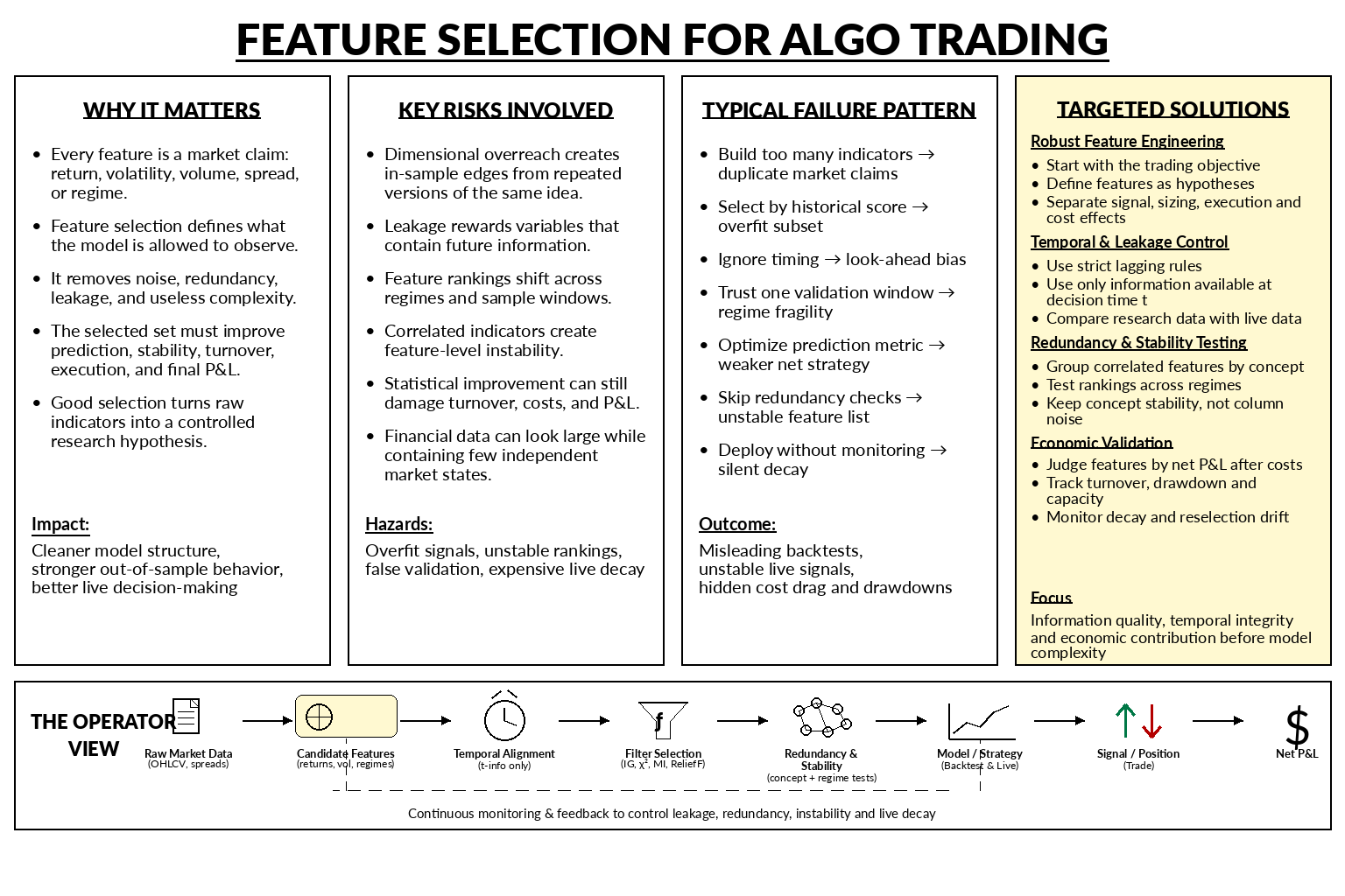
Financial markets produce mountains of data, spanning simple price movements to limit order book dynamics. A common misconception assumes a larger dataset guarantees superior predictions. Reality proves the opposite. Excessive variables introduce noise, and invite to overfitting.
Every input added to a model represents a specific market hypothesis. Including a volatility metric implies price instability shapes future returns. Adding a spread feature connects liquidity to transaction costs. The selection process goes further than basic data preprocessing to become the core architectural decision of a trading system. The target variable dictates the necessary inputs, and aligning these inputs with actual market execution determines strategy success.
High-dimensional environments carry distinct dangers, exposing models to feature leakage, dimensional overreach, and selection instability. A feature might improve a statistical score in a backtest but erode capital in live trading due to increased turnover or delayed entries.
Go deeper in this topic by checking this presentation:
Let’s outline the mechanics and limitations of distinct statistical filters, including Information Gain, Chi-Square tests, Fisher Scores, ANOVA, and Mutual Information. Each method offers a unique lens for evaluating data, from measuring entropy reduction to capturing non-linear dependencies.
What is feature selection?
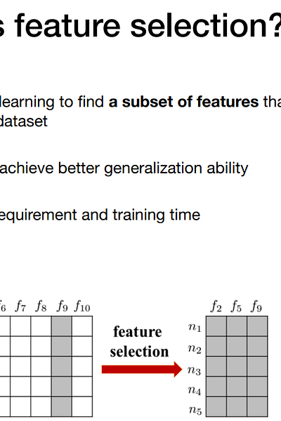
Feature selection is the process of deciding which variables deserve to enter a model and which variables should stay outside it. For example:
A return feature embeds the claim that recent price movement contains information about future outcomes.
A volatility feature treats the magnitude and instability of price movement as relevant to the future distribution of returns.
A volume feature assumes that participation carries informational value.
A spread feature connects liquidity conditions to execution quality, transaction costs, and the practical usefulness of a signal.
A regime feature formalizes the idea that market behavior changes across states.
Therefore, feature selection gives structure to the model. It separates useful information from noise, redundancy, leakage, and unnecessary complexity. A model can receive hundreds of possible inputs, while only a smaller group contributes to consistent performance. Its purpose is to reduce the model’s information set to the variables that improve prediction, reduce instability, and improve the final performance.

The point here is to know which variables remain useful when the model trades under live conditions. A selected feature must contribute beyond other similar variables and survive different market periods. Let us start with the feature set X = {x1, x2, …, xp}.
The problem can be stated simply. The original dataset contains (p) candidate features, each one representing a possible source of information for the model. Feature selection looks for a smaller subset S ⊂ X.
The objective is to choose (S) so the model performs better, generalizes better, and remains easier to monitor. In fact, performance must be measured through the full chain:
Then, a feature becomes valuable when it improves that chain. Conversely, a feature loses value when it improves a statistical score while weakening the final PnL. For example, a feature may improve directional accuracy from 51 percent to 52 percent. At first, that looks useful. Yet if the feature doubles turnover, increases transaction costs, and creates late entries, the strategy becomes weaker. Another feature may show only moderate predictive power, but it may reduce false entries during high-volatility periods. That feature becomes more valuable because it improves the strategy where losses usually appear.
This is why feature selection in follows a higher standard than ordinary data science. In many machine learning problems, the main question is predictive accuracy (that includes recall and F1). But in trading, the question is broader. The model needs useful predictions, stable signals, controlled turnover, and realistic execution across time.
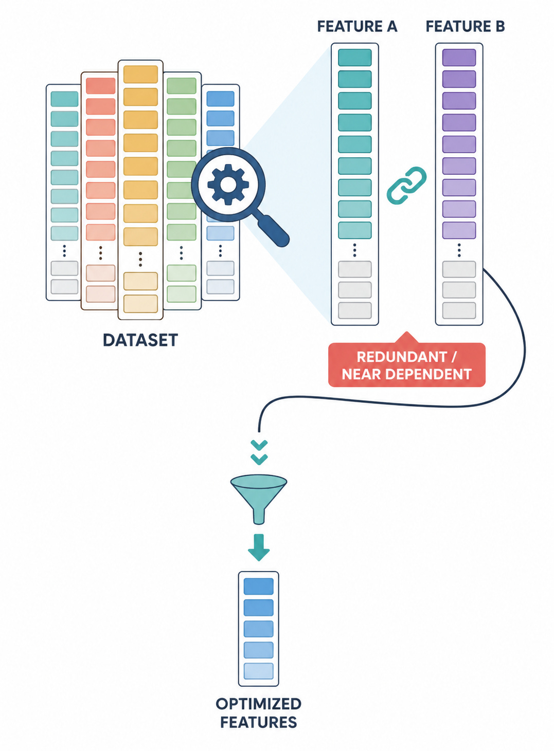
Feature selection also protects the model from redundancy. Many variables express the same idea in different forms. A 5-day return, a 10-day momentum score, a moving-average slope, and a breakout distance may all describe directional pressure. Adding all of them can make the dataset look richer, while the model receives repeated exposure to the same underlying signal.
There are several common ways to select features. Low-variance filters remove variables that barely change. Univariate methods rank each feature by its individual relationship with the target. Recursive feature elimination repeatedly removes weaker variables from a model. L1 regularization pushes weak coefficients toward zero. Tree-based methods estimate which variables help nonlinear decisions. Sequential feature selection adds or removes variables based on their contribution to validation performance.
Feature selection is therefore both a modeling technique and a research control mechanism.

Risks and limitations of feature selection
As stated earlier, a broader feature set gives a model a richer pool for describing market structure. It expands the number of ways in which the model can represent volatility, direction, liquidity, regime behavior, cross-asset transmission, and conditional response. However, every additional feature gives the model another opportunity to attach meaning to patterns that may belong only to the accidental geometry of the sample.
Each feature therefore carries a hypothesis, and a failure mode. Let’s see these costs:
The first risk is dimensional overreach. A model with too many variables can produce excellent in-sample performance while increasing out-of-sample overfitting. This risk grows when the research process tests many transformations of the same underlying idea. A dataset may contain RSI 7, RSI 14, RSI 21, stochastic oscillators, z-scored returns, rolling quantiles, rolling ranks, and several normalized momentum measures. On the research dataframe, this appears diversified. But in market terms, it may express the same directional claim several times under different names.
This is one of the central traps of high-dimensional research. The number of variables grows faster than the number of independent market states. As the feature space expands, the probability of discovering a convincing but empty relationship increases.
The second risk is feature leakage. Leakage appears when a feature contains information that was unavailable at the moment of decision. This problem often appears in subtle forms. For example, a rolling statistic may include the current bar close while the simulated trade is placed at the open; or a volatility estimate may rely on high and low values that occur only after the entry decision.
Feature selection magnifies this problem because selection methods reward the variables that appear most predictive. It improves the validation score, stabilizes the equity curve, and gives the model an artificial sense of intelligence. The problem is that this intelligence is simply overfitting.
The third risk is selection instability. A feature can rank highly in one period, lose relevance in another, and return later. This behavior reflects regime dependence, sample noise, and structural decay. In fact, it sits close to the boundary between usefulness and randomness.
A feature that wins inside a backtest could lose practical value during live conditions. The apparent ranking of features can shift when the research process moves from statistical prediction to executable trading. A variable that improves a model score may still damage the strategy when placed inside the full execution chain.
The fourth risk is economic irrelevance. A feature can improve a statistical metric while weakening the actual trading system. It can raise accuracy from 51.0 percent to 51.5 percent and still reduce profitability when it increases turnover, or concentrates trades. In trading, every feature must be evaluated through its final contribution to the PnL because predictive usefulness alone is insufficient.
Feature selection is designed to reduce the model to useful information, yet the act of selecting features can itself become a source of bleeding money. The researcher uses feature selection to control complexity, but the selection process also needs its own control mechanism. Therefore, it requires more than ranking variables by historical usefulness. The feature set must remain coherent across time, robust under small perturbations, and aligned with the strategy’s market hypothesis.

Feature selection as a research problem
Feature selection can appear mechanical when it is presented as a catalogue of techniques. It creates the impression that a researcher can pass a dataset through a set of filters and obtain, at the end of the process, a smaller and more useful information set.
This impression is attractive because it transforms a difficult research decision into an apparently technical routine. However, the problem is a little bit more complex than that. Feature selection is a research problem because every feature represents a claim about future market behavior.
A lagged return claims that recent price movement contains useful information, while a volatility estimate claims that the current distribution of movement changes the next decision. There are tons of assumptions related to that, like those related to liquidity, cross-asset variable, regime variable and so on.
Selecting a feature therefore means selecting a market hypothesis.
This changes the role of feature selection completely. The researcher is reducing the number of columns in a dataset and deciding what the model is allowed to observe. That choice defines the structure of the model before the model begins to learn. A feature set with many versions of the same idea gives the model a narrow view expressed through many columns.
The first major challenge is temporal order. Trading data arrives through time. The researcher stands at time t, observes only the information available at time t, makes a decision for time t+1 or later, and receives the result only after the market has moved and after trading costs have entered the calculation. This structure changes the entire selection problem.
A feature used at time t must belong to the information set available at time t. The structure can be written as:
The position then follows from the selected information:
The future outcome appears only after the decision:
where qt is the position, rt,t+h is the future return over the holding horizon, and Ct represents commissions, spread, slippage, latency, etc. This small structure captures the essence of the trading problem. The model receives information, takes exposure, and earns a net result. Feature selection must improve that entire chain. This is why time alignment becomes central. The method may look correct while the experiment becomes false. The correctness lives in the timing of information.
The second major challenge comes from the target. In many ordinary prediction problems, the target has a direct definition. In trading, the target is a design decision: next-bar return, next-day return, probability of a positive close, volatility-adjusted return, maximum favorable excursion, maximum adverse excursion, triple-barrier outcome, trend continuation, mean-reversion response, drawdown-conditioned payoff, or expected return after costs. And a pretty long list where each target asks the features a different question.
For this reason, feature selection has to start with the trading objective, not with the dataset. Predicting next-day direction requires one type of information. Sizing exposure from volatility-adjusted expected return requires another. Trend continuation depends on evidence of persistence, while mean reversion depends on evidence of displacement and exhaustion. The same column can carry alpha in one objective and become almost useless in another.
For example, realized volatility may rank highly when the target is absolute return yt=|rt+1|. The same feature may rank much lower when the target is signed return yt=rt+1
Feature correlation is also a major challenge. Different selection methods react to correlation in different ways. This creates a practical problem because the selected feature list can change across time even when the underlying market idea remains stable. One month the model selects a five-day return and another month it selects a moving-average slope. The names change, while the concept remains close to the same directional signal. A shallow reading calls the model unstable. But it is just feature-level instability—from concept-level stability.
Due to all of that financial datasets can look large while containing limited independent information. Intraday data may contain millions of rows, yet many of those rows repeat the same session structure. Daily data may cover decades, yet it still contains a limited number of cycles, liquidity contractions, and structural breaks. The number of rows can exaggerate the amount of independent evidence.
The researcher therefore needs two forms of data sufficiency:
The first is observation count. The feature has to appear often enough for its relationship with the target to be estimated.
The second is regime coverage. The feature has to experience enough different market states for its survival to be tested.
A feature that performs across calm sessions, volatile sessions, gap sessions, trend days, reversal days… carries stronger evidence than a feature that performs in one narrow environment.
Feature selection does not work in isolation. Its value depends on the model that reads the features and the trading objective they are meant to serve. Each method reveals a different part of the picture, and the decision becomes stronger when those signals are interpreted together rather than treated as separate answers.
A prediction eventually has to become an order. That transition changes the evaluation because a feature can improve a prediction metric while weakening the final strategy. For this reason, feature selection must be judged by its effect on realized trading outcomes.

Filter-based feature selection
The curse of dimensionality presents a constant threat to model generalization. When designing trading models, researchers typically construct hundreds or thousands of candidate features from raw limit order book data, transaction flows, technical indicators, and macroeconomic series. Including redundant or uninformative variables accelerate overfitting, and degrades out-of-sample performance.
This is compounded by the low signal-to-noise ratio characteristic of financial markets, where genuine predictive signals are often buried under overwhelming market noise. If a model with high capacity (such as a deep neural network or a gradient-boosted tree) is fed an excessive number of noisy features, it will exploit spurious in-sample correlations, leading to capital loss during live deployment.
Filter-based methods are computationally efficient and model-agnostic. They evaluate the intrinsic statistical properties of individual candidate features relative to a target label—independent of the downstream training phase. This decoupling prevents the leakage of model-specific assumptions and acts as the first line of defense against data-snooping biases.
Information Gain
Information Gain measures the expected reduction in Shannon entropy achieved by partitioning a dataset according to a given feature. Features are often continuous (such as rolling price volatility or volume imbalance), while target variables can be formulated as binary classifications (such as the directional sign of the next N-period return).
Let Y represent the target variable (e.g., Y ∈ {+1, -1}) and X represent a feature. The Shannon entropy of the target H(Y), which quantifies its prior uncertainty, is defined as:
Under non-stationary market conditions, the prior probabilities p(y) of directional movement can shift, altering the baseline entropy. If X is a continuous feature, it must be discretized into K bins to compute the probability distributions over a discrete space. The conditional entropy of Y given X, representing the remaining uncertainty of Y after observing X, is defined as:
Information Gain IG(Y, X) is the absolute difference between these two entropy measures:
A higher IG(Y, X) indicates that observing feature X provides substantial predictive information regarding the market direction. However, the discretization process introduces a critical trade-off. Choosing an equal-width binning strategy can cluster heavy-tailed financial returns into single bins, whereas an equal-frequency (quantile-based) binning strategy preserves distribution density but may dilute local threshold signals.
Assume Y corresponds to whether the next daily return exceeds a transaction-cost threshold. When discretized, Information Gain isolates which thresholds of the indicator carry maximum predictive capacity.
For instance, rather than assuming a linear relationship, IG can identify values that yield a massive drop in the conditional entropy of directional returns, capturing localized non-linear regime behaviors that traditional linear models overlook.
import numpy as np
import pandas as pd
import matplotlib.pyplot as plt
from scipy.stats import entropy

def calculate_entropy(probabilities):
    return entropy(probabilities, base=2)

def information_gain(feature, target, bins=10):
    # Discretize continuous feature
    discretized_feature = pd.qcut(feature, q=bins, labels=False, duplicates='drop')

    # Prior entropy of target
    target_probs = pd.Series(target).value_counts(normalize=True).values
    h_y = calculate_entropy(target_probs)

    # Conditional entropy
    df = pd.DataFrame({'feature': discretized_feature, 'target': target})
    h_y_given_x = 0.0
    total_samples = len(target)

    for val, group in df.groupby('feature'):
        weight = len(group) / total_samples
        group_probs = group['target'].value_counts(normalize=True).values
        h_y_given_x += weight * calculate_entropy(group_probs)

    return h_y - h_y_given_x

# Synthetic data
np.random.seed(42)
n_samples = 1000
target = np.random.choice([0, 1], size=n_samples) # 0: Down, 1: Up

# Predictive feature
feat_predictive = target * 0.4 + np.random.normal(0, 1, size=n_samples)
# Uninformative feature
feat_noise = np.random.normal(0, 1, size=n_samples)

ig_predictive = information_gain(feat_predictive, target)
ig_noise = information_gain(feat_noise, target)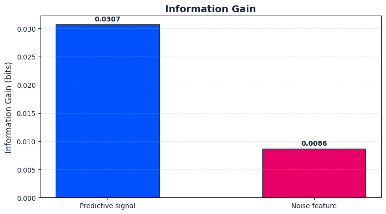
Chi-Square test (X2)
The Chi-Square test of independence assesses whether a categorical feature and a categorical target are statistically independent. Continuous variables are bucketed into categorical regimes to run this test.
The test constructs a contingency table comparing the observed frequency Oij of features and target classes against the expected frequency Eij under the null hypothesis of complete independence:
Where Ri is the sum of row i, Cj is the sum of column j, and N is the total number of observations. The X2 statistic is formulated as:
Higher X2 values indicate a stronger deviation from independence, meaning the feature distribution differs across target classes.
A primary constraint of the X2 test in financial pipelines is its sensitivity to sample sizes and the cell-count distribution. If the target event is a rare tail-risk occurrence, many cells in the contingency table will exhibit expected frequencies Eji < 5. This violation of asymptotic assumptions artificially inflates the Type I error rate, requiring the application of Yates’ correction or Fisher’s Exact Test instead.
Assume we monitor a qualitative state variable, “Is the price above the Upper Bollinger Band?” (Yes/No). We evaluate if this state relates to whether the next trading session experiences a tail-risk event (Drawdown > 2%). A high X2 score confirms that Bollinger Band breakouts carry dependent risk information, allowing risk management systems to adjust leverage based on breakout states.
from scipy.stats import chi2_contingency

def chi_square_score(feature, target, bins=5):
    discretized = pd.qcut(feature, q=bins, labels=False, duplicates='drop')
    contingency_table = pd.crosstab(discretized, target)
    chi2, p_val, _, _ = chi2_contingency(contingency_table)
    return chi2, p_val

# Evaluation
chi2_pred, p_pred = chi_square_score(feat_predictive, target)
chi2_noise, p_noise = chi_square_score(feat_noise, target)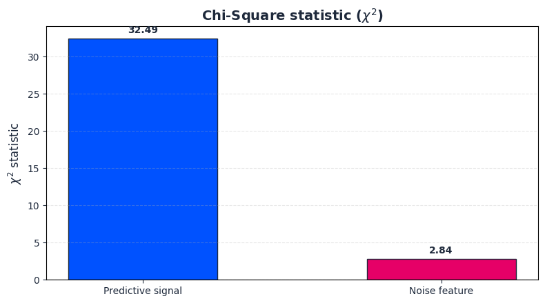
Fisher Score
The Fisher Score is a supervised metric that seeks to maximize the distances between data points of different classes while minimizing the distances between data points within the same class.
For a binary classification target with classes j ∈ {1, 2}, let μji and σ2ji represent the mean and variance of feature i within class j. Let μi represent the global mean of feature i. The Fisher Score Fi for the i-th feature is:
Where nj is the number of samples in class j. A higher Fisher Score implies that the feature’s class-conditional distributions are separated, making it an interesting discriminator.
From a geometric standpoint, the Fisher Score attempts to find features that project the dataset into a space where classes form distinct, compact clusters. However, a significant limitation is that it only evaluates univariate discrimination. If a feature contains multi-modal distributions under a single target class, the mean μji becomes a poor descriptor of central tendency, causing the Fisher Score to severely underestimate the feature’s separation utility.
If a strategy aims to classify market regimes, the Fisher Score evaluates which features show high variation between regimes but low variance within each regime. By prioritizing features with low intra-class variance, the algorithm shields the execution model from volatile signals that might otherwise cause excessive churn.
def fisher_score(feature, target):
    classes = np.unique(target)
    global_mean = np.mean(feature)

    numerator = 0.0
    denominator = 0.0

    for c in classes:
        class_idx = (target == c)
        class_samples = feature[class_idx]
        n_j = len(class_samples)

        mu_ij = np.mean(class_samples)
        var_ij = np.var(class_samples)

        numerator += n_j * (mu_ij - global_mean)**2
        denominator += n_j * var_ij

    return numerator / (denominator + 1e-8)

# Evaluation
fs_pred = fisher_score(feat_predictive, target)
fs_noise = fisher_score(feat_noise, target)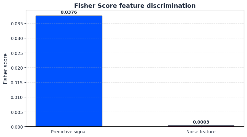
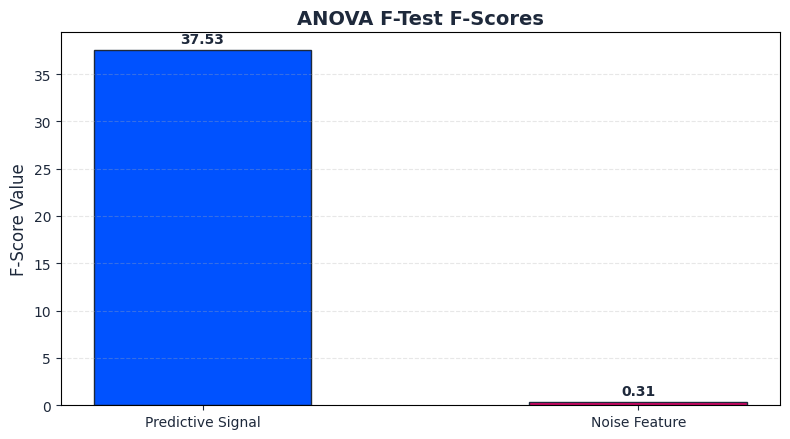
ANOVA F-Test
This test evaluates whether the linear means of a continuous feature differ across several discrete target groups. It is the parametric equivalent to the Fisher Score, built on linear models of variance.
The F-statistic compares the variation between groups (due to class separation) to the variation within groups (unexplained noise):
Where:
k is the number of target classes.
nj is the number of samples in class j.
x̄j is the sample mean of feature X for class j.
x̄ is the overall mean of feature X.
Xij is the value of the feature for the i-th sample in class j.
N is the total sample size.
Under the null hypothesis that all class means are equal, the statistic follows an F-distribution with (k-1, N-k) degrees of freedom.
ANOVA assumes that the residuals within each class are normally distributed and that the groups exhibit homoscedasticity (equal variances). In financial data, these assumptions are violated by fat tails (leptokurtosis) and volatility clustering (autoregressive conditional heteroskedasticity). When these violations occur, the nominal F-statistic can become severely biased, necessitating better alternatives like Welch’s ANOVA.
When predicting discrete regime shifts (e.g., low, medium, or high volatility regimes), ANOVA verifies if the distributions of rolling historic volatilities have statistically distinct averages across these three anticipated states. This ensures that the features selected possess stable, structurally distinct mean levels across different market environments, preventing the trading system from misinterpreting a transient intraday spike as a permanent regime transition.
import numpy as np
from scipy.stats import f


def welch_anova_1d(x, y, eps=1e-12):
    """
    Welch ANOVA for one continuous feature x against a categorical target y.

    It tests whether the class-conditional means of x are different,
    without assuming equal variances across target classes.

    Parameters
    ----------
    x : array-like, shape (n_samples,)
        One continuous feature.

    y : array-like, shape (n_samples,)
        Categorical target labels.

    eps : float
        Small numerical stabilizer for zero variances.

    Returns
    -------
    F_stat : float
        Welch ANOVA F-statistic.

    p_value : float
        P-value from the approximate F distribution.

    df1 : float
        Numerator degrees of freedom.

    df2 : float
        Denominator degrees of freedom.
    """

    x = np.asarray(x, dtype=float)
    y = np.asarray(y)

    classes = np.unique(y)
    k = len(classes)

    if k < 2:
        raise ValueError("Welch ANOVA requires at least two target classes.")

    means = []
    variances = []
    counts = []

    for cls in classes:
        group = x[y == cls]
        group = group[np.isfinite(group)]

        if len(group) < 2:
            raise ValueError("Each class must contain at least two valid observations.")

        means.append(np.mean(group))
        variances.append(np.var(group, ddof=1))
        counts.append(len(group))

    means = np.asarray(means)
    variances = np.asarray(variances)
    counts = np.asarray(counts)

    variances = np.maximum(variances, eps)

    # Welch weights
    weights = counts / variances
    weight_sum = np.sum(weights)

    # Weighted grand mean
    weighted_mean = np.sum(weights * means) / weight_sum

    # Numerator term
    numerator = np.sum(weights * (means - weighted_mean) ** 2) / (k - 1)

    # Welch correction term
    correction_terms = ((1.0 - weights / weight_sum) ** 2) / (counts - 1)
    correction_sum = np.sum(correction_terms)

    denominator = 1.0 + (2.0 * (k - 2) / (k**2 - 1.0)) * correction_sum

    F_stat = numerator / denominator

    df1 = k - 1
    df2 = (k**2 - 1.0) / (3.0 * correction_sum)

    p_value = f.sf(F_stat, df1, df2)

    return F_stat, p_value, df1, df2


def welch_anova_feature_selection(X, y):
    """
    Applies Welch ANOVA to every feature column in X.

    Parameters
    ----------
    X : array-like, shape (n_samples, n_features)
        Feature matrix.

    y : array-like, shape (n_samples,)
        Categorical target.

    Returns
    -------
    f_scores : ndarray
        Welch ANOVA F-statistics for each feature.

    p_values : ndarray
        P-values for each feature.

    df1_values : ndarray
        Numerator degrees of freedom for each feature.

    df2_values : ndarray
        Denominator degrees of freedom for each feature.
    """

    X = np.asarray(X, dtype=float)
    y = np.asarray(y)

    n_features = X.shape[1]

    f_scores = np.zeros(n_features)
    p_values = np.zeros(n_features)
    df1_values = np.zeros(n_features)
    df2_values = np.zeros(n_features)

    for i in range(n_features):
        F_stat, p_value, df1, df2 = welch_anova_1d(X[:, i], y)

        f_scores[i] = F_stat
        p_values[i] = p_value
        df1_values[i] = df1
        df2_values[i] = df2

    return f_scores, p_values, df1_values, df2_values

X_filter = np.column_stack([feat_predictive, feat_noise])

welch_f_scores, welch_p_values, df1_values, df2_values = welch_anova_feature_selection(X_filter, target)
Mutual Information
Unlike linear correlation, Mutual Information (MI) measures both linear and non-linear statistical dependencies between a feature and a target. It determines how much information about the target is shared by the feature.
For a continuous feature X and a discrete target Y, Mutual Information is computed using entropy reduction formulations over continuous spaces:
Estimating continuous probability densities p(x) from finite, noisy financial series is difficult to kernel density bandwidth choices. To mitigate this discretization bias, modern implementations employ k-nearest neighbor (k-NN) entropy estimators (specifically the Kraskov-Stögbauer-Grassberger, or KSG, method).
The KSG framework computes distances to the k-th nearest neighbor in the joint space and marginal spaces, adjusting the MI estimate based on local data density. This prevents the underestimation of information in regions of sparse data, such as market tail events. If a feature has a U-shaped relationship with returns (for instance, extreme values of trading volume indicating potential reversals regardless of direction), standard correlation might yield zero.
Mutual Information identifies this non-linear predictive power. By capturing these relationships, MI allows quantitative researchers to preserve features that signal upcoming volatility expansions or regime turnarounds, even if they show zero linear correlation with price direction.
from sklearn.feature_selection import mutual_info_classif

# Compute Mutual Information
mi_scores = mutual_info_classif(np.column_stack([feat_predictive, feat_noise]), target, random_state=42)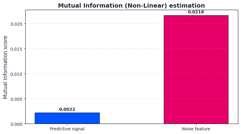
If you look closely, this is the only technique that identifies very little signal and labels most features as noise.
Correlation with target
Linear correlation is the most widely used baseline filter technique due to its simplicity, speed of computation, and intuitive interpretation.
The Pearson product-moment correlation coefficient pX,Y measures the linear relationship between a feature X and a target Y:
For non-normal distributions or monotonic, non-linear dependencies, Spearman’s rank correlation ps is used:
Where di is the difference between the ranks of corresponding variables.
While linear correlation is computationally efficient, it suffers from two major vulnerabilities in time-series trading:
Look-ahead and spurious correlation: Standard correlation is susceptible to outliers. A single extreme market spike can inflate the Pearson score of an otherwise useless feature.
Structural breaks: Financial correlation is dynamic. A feature showing a correlation of +0.15 during a bull market may switch to -0.30 during a liquidity crisis, rendering a static correlation filter dangerous if not computed over rolling windows.
For directional alpha models with a continuous target (such as forward 1-hour returns), a correlation filter screens out technical or fundamental signals with absolute linear correlation values near zero.
It is common to run Spearman correlation filters in parallel with Pearson filters. While Pearson screens for immediate linear predictability, Spearman evaluates if ordinal monotonic patterns exist, ensuring that non-linear but rank-preserving features (such as order book depth rankings) are preserved for downstream tree-based models.
from scipy.stats import pearsonr

# Compute Pearson Correlation
corr_pred, _ = pearsonr(feat_predictive, target)
corr_noise, _ = pearsonr(feat_noise, target)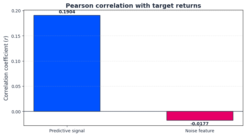
ReliefF
The ReliefF algorithm is a distance-based feature estimator that accounts for feature interactions. It evaluates features based on how well their values distinguish between instances that are near to each other in the multi-dimensional feature space.
ReliefF randomly selects an instance Ri, then searches for its k-nearest neighbors from the same class (called nearest hits Hj) and from the opposite class (called nearest misses Mj(C)). It updates the weight of each feature A as follows:
Where:
diff(A, I1, I2) computes the normalized difference in feature A between instances I1 and I2.
m is the number of random instances sampled.
P(C) is the prior probability of class C.
The selection of the metric used to calculate the nearest neighbors is critical. While Euclidean distance is common, the Manhattan metric is preferred in higher-dimensional spaces to mitigate the concentration of measure phenomenon, where distances between points collapse to a uniform value.
In fact, the hyperparameter k (number of neighbors) acts as a low-pass filter. A small k captures fine-grained local dependencies but is sensitive to outlier trades, while a large k smooths out noise but risks washing out localized, fleeting edge conditions.
If two features are only predictive when combined (such as volatility and volume acting together as a structural marker of liquidations), traditional univariate filters will miss them. ReliefF captures these joint localized geometric dependencies.
For instance, ReliefF can identify that while “order book depth” and “volatility” could be mediocre predictors on their own, their localized configuration during market-maker pullbacks separates profitable long entries from fake-outs.
from sklearn.neighbors import NearestNeighbors

def simplified_relieff(X, y, n_neighbors=5, n_samples=200):
    n_inst, n_feats = X.shape
    weights = np.zeros(n_feats)

    # Fit nearest neighbors per class
    classes = np.unique(y)
    nn_dict = {}
    for c in classes:
        nn = NearestNeighbors(n_neighbors=n_neighbors + 1, metric='manhattan')
        nn.fit(X[y == c])
        nn_dict[c] = nn

    # Sample index selection
    rng = np.random.default_rng(42)
    sample_indices = rng.choice(n_inst, size=min(n_samples, n_inst), replace=False)

    for idx in sample_indices:
        inst = X[idx]
        label = y[idx]

        # Hit search: same class
        # Drop first match because it might be the query point itself
        dists_hit, indices_hit = nn_dict[label].kneighbors([inst])
        hits = X[y == label][indices_hit[0][1:]]

        # Miss search: different classes
        misses_dict = {}
        for c in classes:
            if c == label:
                continue
            dists_miss, indices_miss = nn_dict[c].kneighbors([inst])
            misses_dict[c] = X[y == c][indices_miss[0][1:]]

        for f in range(n_feats):
            # Compute difference to hits
            diff_hit = np.mean(np.abs(inst[f] - hits[:, f]))

            # Compute difference to misses
            diff_miss = 0.0
            for c, misses in misses_dict.items():
                diff_miss += np.mean(np.abs(inst[f] - misses[:, f]))

            weights[f] = weights[f] - diff_hit + diff_miss

    return weights / n_samples

# Setup dataset matrix
X_matrix = np.column_stack([feat_predictive, feat_noise])
# Min-max scale columns prior to ReliefF
X_scaled = (X_matrix - X_matrix.min(axis=0)) / (X_matrix.max(axis=0) - X_matrix.min(axis=0))

relieff_weights = simplified_relieff(X_scaled, target)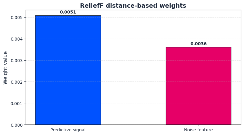
Minimum Redundancy Maximum Relevance (mRMR)
The mRMR algorithm optimizes feature selection by addressing a key limitation of univariate filters (the selection of mutually redundant features). It searches for a feature subset that has high correlation with the target (maximum relevance) but low correlation among the selected features themselves (minimum redundancy).
Let S represent the subset of selected features, Y represent the target, and I(X; Y) denote the Mutual Information between feature X and target Y. The optimization problem is defined as:
Where:
Under the standard Mutual Information Difference scheme, the next feature Xk is selected from the candidate set X \ S by maximizing:
An alternative configuration is the Mutual Information Quotient scheme, which defines the selection criterion ratio-metrically:
Where ε is a small regularization constant to prevent division by zero. While MID penalizes redundancy linearly, MIQ penalizes it scale-metrically. In trading systems where features exhibit intense, multi-scale collinearity (such as overlapping moving averages), the ratio-metric MIQ is often more stable, preventing a predictive but redundant feature from being suppressed by a large set of weakly redundant variables.
A model might find that rolling historical 5-day, 10-day, and 15-day volatilities all have high individual relevance to forward market returns. However, choosing all three is pretty redundant. mRMR will select the most relevant volatility window first, then penalize the others due to their high mutual information, forcing the system to select an independent feature (such as order flow imbalance or funding rates) instead.
This diversification across feature modalities is crucial for building multi-asset or systematic trend-following strategies, as it directly restricts the feature space from collapsing into a single, correlated risk exposure.
import numpy as np
import matplotlib.pyplot as plt

from sklearn.feature_selection import mutual_info_classif, mutual_info_regression


def mrmr_select_one_next(X, y, selected_indices, candidates_indices, task="classification"):
    """
    Selects the next best feature using the MID variant of mRMR:

        score(x_i) = I(x_i ; y) - mean_j I(x_i ; x_j)

    where:
        I(x_i ; y)   = relevance
        I(x_i ; x_j) = redundancy

    Parameters
    ----------
    task : {"classification", "regression"}
        - "classification": y is discrete, e.g. 0/1.
        - "regression": y is continuous, e.g. future returns.
    """

    n_selected = len(selected_indices)

    def relevance_mi(i):
        if task == "classification":
            return mutual_info_classif(
                X[:, [i]],
                y,
                random_state=42
            )[0]
        elif task == "regression":
            return mutual_info_regression(
                X[:, [i]],
                y,
                random_state=42
            )[0]
        else:
            raise ValueError("task must be either 'classification' or 'regression'")

    def redundancy_mi(i, j):
        # Feature-feature MI is continuous-continuous,
        # therefore use mutual_info_regression.
        return mutual_info_regression(
            X[:, [i]],
            X[:, j],
            random_state=42
        )[0]

    if n_selected == 0:
        relevances = [relevance_mi(i) for i in candidates_indices]
        best_cand = candidates_indices[np.argmax(relevances)]
        return best_cand, np.max(relevances)

    best_score = -np.inf
    best_cand = None

    for i in candidates_indices:
        relevance = relevance_mi(i)

        redundancy = 0.0
        for j in selected_indices:
            redundancy += redundancy_mi(i, j)

        redundancy /= n_selected

        score = relevance - redundancy

        if score > best_score:
            best_score = score
            best_cand = i

    return best_cand, best_score

# Construct synthetic multi-feature collinear matrix
# Feature 0: High predictive capacity
# Feature 1: Highly redundant to Feature 0
# Feature 2: High noise, completely uncorrelated
feat_collinear = feat_predictive * 0.95 + np.random.normal(0, 0.1, size=n_samples)
X_multivariate = np.column_stack([feat_predictive, feat_collinear, feat_noise])

# Iterative mRMR selection
selected = []
candidates = [0, 1, 2]
mrmr_scores = []

for step in range(3):
    best, score = mrmr_select_one_next(X_multivariate, target, selected, candidates)
    selected.append(best)
    candidates.remove(best)
    mrmr_scores.append((best, score))

# Output display data format
names_map = {0: "Predictive", 1: "Redundant", 2: "Noise"}
selection_order = [names_map[idx] for idx, _ in mrmr_scores]
scores_recorded = [score for _, score in mrmr_scores]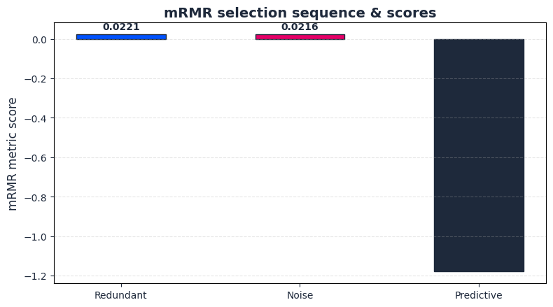
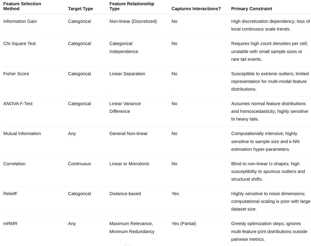
The choice of filter method should be tailored to the underlying structure of the feature candidate set, target variable constraints, and assumptions about model linearities.

Alright! Amazing work today, everyone! Maybe this message should have come earlier, but that’s how it goes. Better late than never. Time to wrap it up. Stay sharp, stay fearless, stay moving forward 🚀
PS: Hey guys! Give me feedback for the newsletter and this topic (feature selection):
This is an invitation-only access to our QUANT COMMUNITY, so we verify numbers to avoid spammers and scammers. Feel free to join or decline at any time. Tap the WhatsApp icon below to join

Appendix
Full Script
from __future__ import annotations

from dataclasses import dataclass
from typing import Iterable, Literal, Sequence

import numpy as np
import pandas as pd
from scipy.stats import chi2_contingency, entropy, f, pearsonr
from sklearn.feature_selection import f_classif, mutual_info_classif, mutual_info_regression
from sklearn.neighbors import NearestNeighbors


TaskType = Literal["classification", "regression"]

# General utilities

def _as_2d_float_array(X: np.ndarray | Sequence[Sequence[float]]) -> np.ndarray:
    X_arr = np.asarray(X, dtype=float)

    if X_arr.ndim == 1:
        X_arr = X_arr.reshape(-1, 1)

    if X_arr.ndim != 2:
        raise ValueError("X must be a 1D or 2D array.")

    return X_arr


def _as_1d_array(y: np.ndarray | Sequence) -> np.ndarray:
    y_arr = np.asarray(y)

    if y_arr.ndim != 1:
        raise ValueError("y must be a 1D array.")

    return y_arr


def _clean_feature_target(
    feature: np.ndarray | Sequence[float],
    target: np.ndarray | Sequence,
) -> tuple[np.ndarray, np.ndarray]:
    x = np.asarray(feature, dtype=float)
    y = _as_1d_array(target)

    if x.ndim != 1:
        raise ValueError("feature must be a 1D array.")

    if len(x) != len(y):
        raise ValueError("feature and target must have the same length.")

    mask = np.isfinite(x) & pd.notna(y)
    x = x[mask]
    y = y[mask]

    if len(x) == 0:
        raise ValueError("No valid observations after removing NaN/inf values.")

    return x, y


def _quantile_discretize(feature: np.ndarray, bins: int = 10) -> np.ndarray:
    """
    Discretize a continuous feature into quantile bins.

    This keeps the filter methods usable for continuous trading features such as
    volatility, spread, range, momentum, distance to VWAP, z-score, etc.
    """
    if bins < 2:
        raise ValueError("bins must be >= 2.")

    x = np.asarray(feature, dtype=float)

    if np.unique(x).size <= 1:
        return np.zeros(len(x), dtype=int)

    discretized = pd.qcut(
        x,
        q=min(bins, np.unique(x).size),
        labels=False,
        duplicates="drop",
    )

    codes = pd.Series(discretized).fillna(0).astype(int).to_numpy()
    return codes


def minmax_scale(X: np.ndarray | Sequence[Sequence[float]], eps: float = 1e-12) -> np.ndarray:
    """
    Min-max scale every feature column.

    ReliefF is distance-based, so scaling is important.
    """
    X_arr = _as_2d_float_array(X)

    mn = np.nanmin(X_arr, axis=0)
    mx = np.nanmax(X_arr, axis=0)

    return (X_arr - mn) / np.maximum(mx - mn, eps)


# 1. Information Gain

def calculate_entropy(probabilities: np.ndarray | Sequence[float]) -> float:
    """
    Shannon entropy in base 2.
    """
    probabilities = np.asarray(probabilities, dtype=float)
    probabilities = probabilities[probabilities > 0.0]

    if len(probabilities) == 0:
        return 0.0

    return float(entropy(probabilities, base=2))


def information_gain(
    feature: np.ndarray | Sequence[float],
    target: np.ndarray | Sequence,
    bins: int = 10,
) -> float:
    """
    Information Gain:

        IG(X;Y) = H(Y) - H(Y|X)

    For continuous features, X is discretized into quantile bins.
    """
    x, y = _clean_feature_target(feature, target)
    x_disc = _quantile_discretize(x, bins=bins)

    target_probs = pd.Series(y).value_counts(normalize=True).values
    h_y = calculate_entropy(target_probs)

    df = pd.DataFrame({"feature": x_disc, "target": y})
    h_y_given_x = 0.0
    total_samples = len(df)

    for _, group in df.groupby("feature", observed=True):
        weight = len(group) / total_samples
        group_probs = group["target"].value_counts(normalize=True).values
        h_y_given_x += weight * calculate_entropy(group_probs)

    return float(h_y - h_y_given_x)


def information_gain_scores(
    X: np.ndarray | Sequence[Sequence[float]],
    y: np.ndarray | Sequence,
    bins: int = 10,
) -> np.ndarray:
    X_arr = _as_2d_float_array(X)
    return np.array([information_gain(X_arr[:, i], y, bins=bins) for i in range(X_arr.shape[1])])


# 2. Chi-Square Test

def chi_square_score(
    feature: np.ndarray | Sequence[float],
    target: np.ndarray | Sequence,
    bins: int = 5,
) -> tuple[float, float]:
    """
    Chi-square test between a discretized continuous feature and a categorical target.
    """
    x, y = _clean_feature_target(feature, target)
    x_disc = _quantile_discretize(x, bins=bins)

    contingency_table = pd.crosstab(x_disc, y)

    if contingency_table.shape[0] < 2 or contingency_table.shape[1] < 2:
        return 0.0, 1.0

    chi2, p_value, _, _ = chi2_contingency(contingency_table)
    return float(chi2), float(p_value)


def chi_square_scores(
    X: np.ndarray | Sequence[Sequence[float]],
    y: np.ndarray | Sequence,
    bins: int = 5,
) -> tuple[np.ndarray, np.ndarray]:
    X_arr = _as_2d_float_array(X)

    chi2_values = np.zeros(X_arr.shape[1])
    p_values = np.ones(X_arr.shape[1])

    for i in range(X_arr.shape[1]):
        chi2_values[i], p_values[i] = chi_square_score(X_arr[:, i], y, bins=bins)

    return chi2_values, p_values


# 3. Fisher Score

def fisher_score(
    feature: np.ndarray | Sequence[float],
    target: np.ndarray | Sequence,
    eps: float = 1e-12,
) -> float:
    """
    Fisher score:

        score_j = sum_c n_c (mu_c - mu)^2 / sum_c n_c sigma_c^2

    High values indicate stronger class separation.
    """
    x, y = _clean_feature_target(feature, target)

    classes = np.unique(y)
    global_mean = np.mean(x)

    numerator = 0.0
    denominator = 0.0

    for cls in classes:
        group = x[y == cls]
        n_cls = len(group)

        if n_cls == 0:
            continue

        mu_cls = np.mean(group)
        var_cls = np.var(group)

        numerator += n_cls * (mu_cls - global_mean) ** 2
        denominator += n_cls * var_cls

    return float(numerator / (denominator + eps))


def fisher_scores(
    X: np.ndarray | Sequence[Sequence[float]],
    y: np.ndarray | Sequence,
) -> np.ndarray:
    X_arr = _as_2d_float_array(X)
    return np.array([fisher_score(X_arr[:, i], y) for i in range(X_arr.shape[1])])


# 4. Standard ANOVA F-Test

def anova_f_scores(
    X: np.ndarray | Sequence[Sequence[float]],
    y: np.ndarray | Sequence,
) -> tuple[np.ndarray, np.ndarray]:
    """
    Standard ANOVA F-test from scikit-learn.

    This assumes equal variance across target classes, so it is less robust than
    Welch ANOVA when the market regimes/classes have different dispersion.
    """
    X_arr = _as_2d_float_array(X)
    y_arr = _as_1d_array(y)

    f_scores, p_values = f_classif(X_arr, y_arr)

    return np.asarray(f_scores, dtype=float), np.asarray(p_values, dtype=float)


# 5. Welch ANOVA

def welch_anova_1d(
    feature: np.ndarray | Sequence[float],
    target: np.ndarray | Sequence,
    eps: float = 1e-12,
) -> tuple[float, float, float, float]:
    """
    Welch ANOVA for one continuous feature against a categorical target.

    It tests whether class-conditional means differ without assuming equal
    variances across classes.
    """
    x, y = _clean_feature_target(feature, target)

    classes = np.unique(y)
    k = len(classes)

    if k < 2:
        raise ValueError("Welch ANOVA requires at least two target classes.")

    means = []
    variances = []
    counts = []

    for cls in classes:
        group = x[y == cls]
        group = group[np.isfinite(group)]

        if len(group) < 2:
            raise ValueError("Each target class must contain at least two valid observations.")

        means.append(np.mean(group))
        variances.append(np.var(group, ddof=1))
        counts.append(len(group))

    means = np.asarray(means)
    variances = np.maximum(np.asarray(variances), eps)
    counts = np.asarray(counts)

    weights = counts / variances
    weight_sum = np.sum(weights)
    weighted_mean = np.sum(weights * means) / weight_sum

    numerator = np.sum(weights * (means - weighted_mean) ** 2) / (k - 1)

    correction_terms = ((1.0 - weights / weight_sum) ** 2) / (counts - 1)
    correction_sum = np.sum(correction_terms)

    denominator = 1.0 + (2.0 * (k - 2) / (k**2 - 1.0)) * correction_sum

    f_stat = numerator / denominator

    df1 = float(k - 1)
    df2 = float((k**2 - 1.0) / (3.0 * correction_sum))
    p_value = float(f.sf(f_stat, df1, df2))

    return float(f_stat), p_value, df1, df2


def welch_anova_feature_selection(
    X: np.ndarray | Sequence[Sequence[float]],
    y: np.ndarray | Sequence,
) -> tuple[np.ndarray, np.ndarray, np.ndarray, np.ndarray]:
    X_arr = _as_2d_float_array(X)

    f_scores = np.zeros(X_arr.shape[1])
    p_values = np.zeros(X_arr.shape[1])
    df1_values = np.zeros(X_arr.shape[1])
    df2_values = np.zeros(X_arr.shape[1])

    for i in range(X_arr.shape[1]):
        f_scores[i], p_values[i], df1_values[i], df2_values[i] = welch_anova_1d(X_arr[:, i], y)

    return f_scores, p_values, df1_values, df2_values


# 6. Mutual Information

def mutual_information_scores(
    X: np.ndarray | Sequence[Sequence[float]],
    y: np.ndarray | Sequence,
    task: TaskType = "classification",
    random_state: int = 42,
) -> np.ndarray:
    """
    Mutual Information between every feature and the target.

    Classification:
        I(feature ; class label)

    Regression:
        I(feature ; continuous target)
    """
    X_arr = _as_2d_float_array(X)
    y_arr = _as_1d_array(y)

    if task == "classification":
        return mutual_info_classif(X_arr, y_arr, random_state=random_state)

    if task == "regression":
        return mutual_info_regression(X_arr, y_arr, random_state=random_state)

    raise ValueError("task must be either 'classification' or 'regression'.")

# 7. Correlation With Target

def pearson_correlation_scores(
    X: np.ndarray | Sequence[Sequence[float]],
    y: np.ndarray | Sequence,
) -> tuple[np.ndarray, np.ndarray]:
    """
    Pearson correlation between every feature and the target.

    For a binary trading target, this measures linear separation between
    up/down outcomes.
    """
    X_arr = _as_2d_float_array(X)
    y_arr = np.asarray(y, dtype=float)

    corr_values = np.zeros(X_arr.shape[1])
    p_values = np.ones(X_arr.shape[1])

    for i in range(X_arr.shape[1]):
        x, y_clean = _clean_feature_target(X_arr[:, i], y_arr)

        if np.unique(x).size <= 1 or np.unique(y_clean).size <= 1:
            corr_values[i] = 0.0
            p_values[i] = 1.0
            continue

        corr_values[i], p_values[i] = pearsonr(x, y_clean)

    return corr_values, p_values


# 8. Simplified ReliefF

def simplified_relieff(
    X: np.ndarray | Sequence[Sequence[float]],
    y: np.ndarray | Sequence,
    n_neighbors: int = 5,
    n_samples: int | None = 200,
    random_state: int = 42,
    scale: bool = True,
) -> np.ndarray:
    """
    Simplified ReliefF.

    Positive weights indicate that nearby samples from different classes are
    far apart while nearby samples from the same class are close.

    This implementation is designed for categorical targets.
    """
    X_arr = _as_2d_float_array(X)
    y_arr = _as_1d_array(y)

    if len(X_arr) != len(y_arr):
        raise ValueError("X and y must have the same number of rows.")

    finite_rows = np.isfinite(X_arr).all(axis=1) & pd.notna(y_arr)
    X_arr = X_arr[finite_rows]
    y_arr = y_arr[finite_rows]

    if scale:
        X_arr = minmax_scale(X_arr)

    n_inst, n_feats = X_arr.shape
    classes = np.unique(y_arr)

    if len(classes) < 2:
        raise ValueError("ReliefF requires at least two target classes.")

    class_indices = {cls: np.where(y_arr == cls)[0] for cls in classes}

    for cls, indices in class_indices.items():
        if len(indices) < 2:
            raise ValueError("Each class must contain at least two observations for ReliefF.")

    rng = np.random.default_rng(random_state)
    sample_size = n_inst if n_samples is None else min(n_samples, n_inst)
    sample_indices = rng.choice(n_inst, size=sample_size, replace=False)

    # Build a nearest-neighbor model for each class.
    nn_models = {}
    class_X = {}

    for cls in classes:
        X_cls = X_arr[class_indices[cls]]
        class_X[cls] = X_cls

        k_cls = min(n_neighbors + 1, len(X_cls))
        nn = NearestNeighbors(n_neighbors=k_cls, metric="manhattan")
        nn.fit(X_cls)
        nn_models[cls] = nn

    weights = np.zeros(n_feats)

    for idx in sample_indices:
        inst = X_arr[idx]
        label = y_arr[idx]

        # Nearest hits: same class. First element is usually the query itself.
        _, hit_indices = nn_models[label].kneighbors([inst])
        hits = class_X[label][hit_indices[0]]

        if len(hits) > 1:
            hits = hits[1:]
        else:
            continue

        hit_diff = np.mean(np.abs(hits - inst), axis=0)

        # Nearest misses: other classes.
        miss_diff = np.zeros(n_feats)
        n_miss_classes = 0

        for cls in classes:
            if cls == label:
                continue

            _, miss_indices = nn_models[cls].kneighbors([inst])
            misses = class_X[cls][miss_indices[0][:n_neighbors]]

            if len(misses) == 0:
                continue

            miss_diff += np.mean(np.abs(misses - inst), axis=0)
            n_miss_classes += 1

        if n_miss_classes > 0:
            miss_diff /= n_miss_classes

        weights += miss_diff - hit_diff

    return weights / sample_size


# 9. Minimum Redundancy Maximum Relevance, MID variant

def _mrmr_relevance_mi(
    X: np.ndarray,
    y: np.ndarray,
    feature_index: int,
    task: TaskType,
    random_state: int,
) -> float:
    if task == "classification":
        return float(
            mutual_info_classif(
                X[:, [feature_index]],
                y,
                random_state=random_state,
            )[0]
        )

    if task == "regression":
        return float(
            mutual_info_regression(
                X[:, [feature_index]],
                y,
                random_state=random_state,
            )[0]
        )

    raise ValueError("task must be either 'classification' or 'regression'.")


def _mrmr_redundancy_mi(
    X: np.ndarray,
    feature_i: int,
    feature_j: int,
    random_state: int,
) -> float:
    """
    Feature-feature MI is continuous-continuous, so mutual_info_regression is used.
    """
    return float(
        mutual_info_regression(
            X[:, [feature_i]],
            X[:, feature_j],
            random_state=random_state,
        )[0]
    )


def mrmr_select_one_next(
    X: np.ndarray | Sequence[Sequence[float]],
    y: np.ndarray | Sequence,
    selected_indices: Sequence[int],
    candidate_indices: Sequence[int],
    task: TaskType = "classification",
    random_state: int = 42,
) -> tuple[int, float]:
    """
    Select the next feature using the MID variant of mRMR:

        score(x_i) = I(x_i ; y) - mean_j I(x_i ; x_j)

    where:
        I(x_i ; y)   = relevance
        I(x_i ; x_j) = redundancy
    """
    X_arr = _as_2d_float_array(X)
    y_arr = _as_1d_array(y)

    selected_indices = list(selected_indices)
    candidate_indices = list(candidate_indices)

    if len(candidate_indices) == 0:
        raise ValueError("candidate_indices cannot be empty.")

    if len(selected_indices) == 0:
        relevances = [
            _mrmr_relevance_mi(X_arr, y_arr, i, task=task, random_state=random_state)
            for i in candidate_indices
        ]
        best_position = int(np.argmax(relevances))
        return candidate_indices[best_position], float(relevances[best_position])

    best_score = -np.inf
    best_candidate = candidate_indices[0]

    for i in candidate_indices:
        relevance = _mrmr_relevance_mi(X_arr, y_arr, i, task=task, random_state=random_state)

        redundancy = np.mean(
            [
                _mrmr_redundancy_mi(X_arr, i, j, random_state=random_state)
                for j in selected_indices
            ]
        )

        score = relevance - redundancy

        if score > best_score:
            best_score = score
            best_candidate = i

    return int(best_candidate), float(best_score)


def mrmr_select_features(
    X: np.ndarray | Sequence[Sequence[float]],
    y: np.ndarray | Sequence,
    k: int,
    task: TaskType = "classification",
    random_state: int = 42,
) -> tuple[list[int], list[float]]:
    """
    Iteratively select k features with mRMR MID.
    """
    X_arr = _as_2d_float_array(X)

    if k < 1:
        raise ValueError("k must be >= 1.")

    k = min(k, X_arr.shape[1])

    selected: list[int] = []
    candidates = list(range(X_arr.shape[1]))
    scores: list[float] = []

    for _ in range(k):
        best, score = mrmr_select_one_next(
            X_arr,
            y,
            selected_indices=selected,
            candidate_indices=candidates,
            task=task,
            random_state=random_state,
        )

        selected.append(best)
        candidates.remove(best)
        scores.append(score)

    return selected, scores


# One-table evaluation helper

@dataclass
class FilterSelectionResult:
    scores: pd.DataFrame
    mrmr_order: pd.DataFrame


def evaluate_all_filter_methods(
    X: np.ndarray | Sequence[Sequence[float]],
    y: np.ndarray | Sequence,
    feature_names: Sequence[str] | None = None,
    bins_information_gain: int = 10,
    bins_chi_square: int = 5,
    relieff_neighbors: int = 5,
    relieff_samples: int | None = 200,
    random_state: int = 42,
) -> FilterSelectionResult:
    """
    Run all supervised filter methods and return:
    - scores table with one row per feature
    - mRMR selection order table
    """
    X_arr = _as_2d_float_array(X)
    y_arr = _as_1d_array(y)

    n_features = X_arr.shape[1]

    if feature_names is None:
        feature_names = [f"feature_{i}" for i in range(n_features)]

    if len(feature_names) != n_features:
        raise ValueError("feature_names must have the same length as the number of columns in X.")

    ig = information_gain_scores(X_arr, y_arr, bins=bins_information_gain)
    chi2_values, chi2_p = chi_square_scores(X_arr, y_arr, bins=bins_chi_square)
    fisher = fisher_scores(X_arr, y_arr)
    anova_f, anova_p = anova_f_scores(X_arr, y_arr)
    welch_f, welch_p, welch_df1, welch_df2 = welch_anova_feature_selection(X_arr, y_arr)
    mi = mutual_information_scores(X_arr, y_arr, task="classification", random_state=random_state)
    pearson_corr, pearson_p = pearson_correlation_scores(X_arr, y_arr)
    relieff = simplified_relieff(
        X_arr,
        y_arr,
        n_neighbors=relieff_neighbors,
        n_samples=relieff_samples,
        random_state=random_state,
        scale=True,
    )

    selected_indices, mrmr_scores = mrmr_select_features(
        X_arr,
        y_arr,
        k=n_features,
        task="classification",
        random_state=random_state,
    )

    scores = pd.DataFrame(
        {
            "feature": list(feature_names),
            "information_gain": ig,
            "chi_square": chi2_values,
            "chi_square_p_value": chi2_p,
            "fisher_score": fisher,
            "anova_f": anova_f,
            "anova_p_value": anova_p,
            "welch_anova_f": welch_f,
            "welch_anova_p_value": welch_p,
            "welch_df1": welch_df1,
            "welch_df2": welch_df2,
            "mutual_information": mi,
            "pearson_corr": pearson_corr,
            "abs_pearson_corr": np.abs(pearson_corr),
            "pearson_p_value": pearson_p,
            "relieff_weight": relieff,
        }
    )

    mrmr_order = pd.DataFrame(
        {
            "rank": np.arange(1, len(selected_indices) + 1),
            "feature_index": selected_indices,
            "feature": [feature_names[i] for i in selected_indices],
            "mrmr_mid_score": mrmr_scores,
        }
    )

    return FilterSelectionResult(scores=scores, mrmr_order=mrmr_order)


# Synthetic trading-style example

def make_synthetic_trading_dataset(
    n_samples: int = 1_000,
    random_state: int = 42,
) -> tuple[np.ndarray, np.ndarray, list[str]]:
    """
    Create a small supervised feature-selection dataset.

    target:
        0 = next bar down
        1 = next bar up

    features:
        predictive_feature = noisy feature with class information
        redundant_feature  = highly collinear version of the predictive feature
        noise_feature      = pure noise
    """
    rng = np.random.default_rng(random_state)

    target = rng.choice([0, 1], size=n_samples)

    predictive_feature = target * 0.40 + rng.normal(0.0, 1.0, size=n_samples)
    redundant_feature = predictive_feature * 0.95 + rng.normal(0.0, 0.10, size=n_samples)
    noise_feature = rng.normal(0.0, 1.0, size=n_samples)

    X = np.column_stack(
        [
            predictive_feature,
            redundant_feature,
            noise_feature,
        ]
    )

    feature_names = [
        "predictive_feature",
        "redundant_feature",
        "noise_feature",
    ]

    return X, target, feature_names


def main() -> None:
    X, y, feature_names = make_synthetic_trading_dataset(
        n_samples=1_000,
        random_state=42,)

    result = evaluate_all_filter_methods(
        X,
        y,
        feature_names=feature_names,
        bins_information_gain=10,
        bins_chi_square=5,
        relieff_neighbors=5,
        relieff_samples=200,
        random_state=42,)

    pd.set_option("display.max_columns", None)
    pd.set_option("display.width", 180)

    print("\n Supervised Filter Scores ")
    print(result.scores.round(6).to_string(index=False))

    print("\n mRMR Selection Order ")
    print(result.mrmr_order.round(6).to_string(index=False))


if __name__ == "__main__":
    main()