

[WITH CODE] Data: Data structures as lifecycle engineering
Lifecycle beats micro-optimization

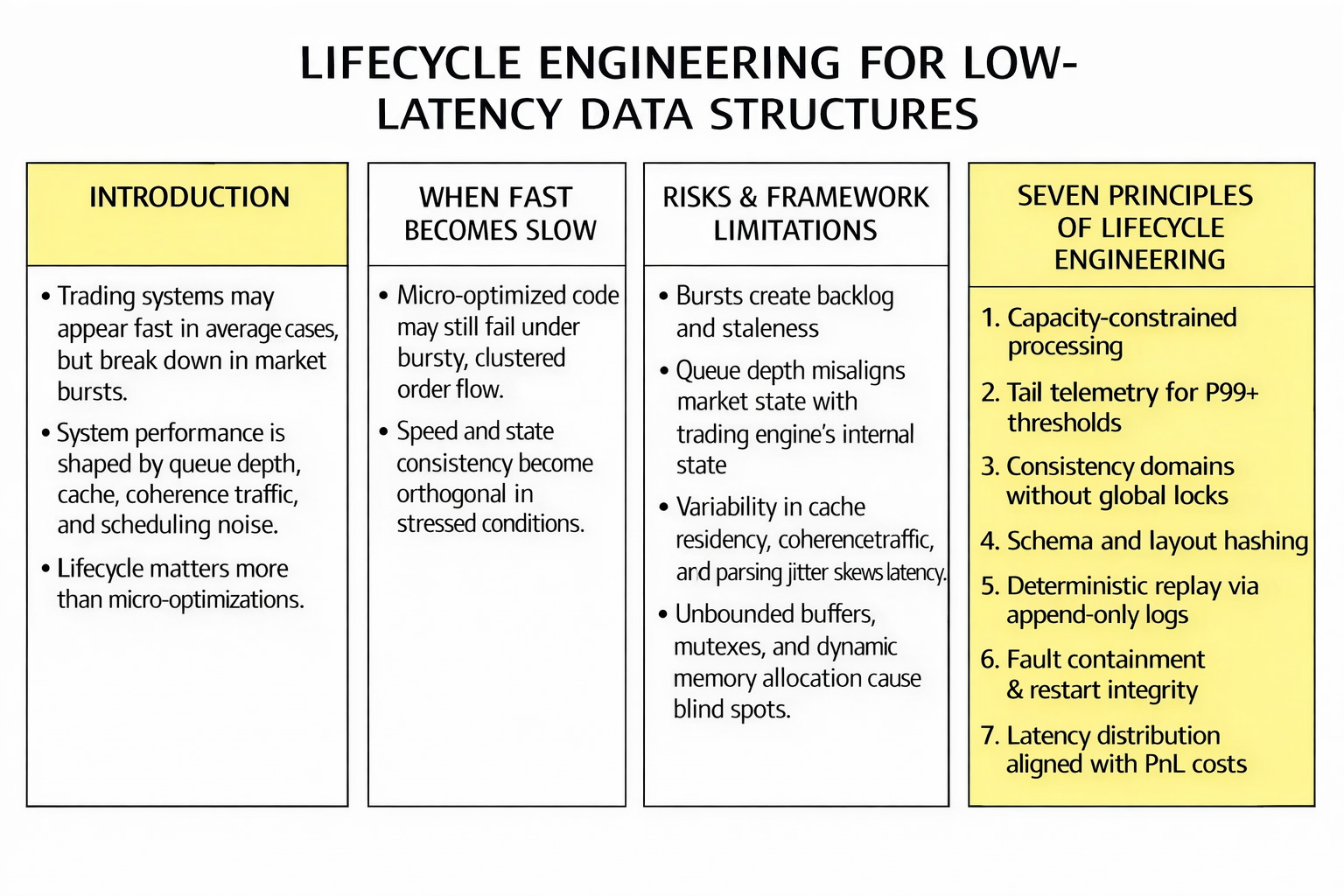
Table of contents:
Introduction.
When fast becomes slow.
Risks and framework limitations.
Lifecycle engineering for low latency data structures.
Point 1 — Capacity-constrained processing.
Point 2 — Tail telemetry.
Point 3 — Consistency domains without global locks.
Point 4 — Schema and layout hashing.
Point 5 — Deterministic replay.
Point 6 — Fault containment, controlled degradation, and restart integrity.
Point 7 — Latency distribution.
Before you begin, remember that you have an index with the newsletter content organized by clicking on “Read the newsletter index” in this image.

Introduction
Most performance failures in trading systems don’t look like failures. You know, impressive microbenchmarks, clean profiles, and average latency that inspire confidence. Then the market compresses time. A volatility microburst lands, the arrival process stops behaving like expected and the engine doesn’t slow down uniformly. One thread stays current, another drifts into backlog, and a third starts making decisions with a reality that no longer exists. This sounds familiar, doesn’t it?
The strategy still runs. Orders still go out. PnL still prints. But the system has quietly crossed a boundary. That boundary is the actual subject of low-latency engineering. Not how fast can you execute a loop, but under what load does your system lose coherence—and what happens to decision quality when it does.
Whether the state you believed you had matches the book you actually traded against. A system that is quick most of the day yet slow precisely during clustered order-flow is not a fast system. The result? The trading system becomes hardware-dependent, shaped by queue depth, cache residency, coherence traffic, parser variability, and scheduling noise. At that point, edge becomes a random variable.
To know more about that, check this:

Today we review more than simple micro-optimizations. Once allocator jitter, false sharing, and accidental copies are tamed, the remaining problem is lifecycle. How is state created, mutated, published, observed, persisted, replayed, and recovered—without letting burst dynamics rewrite the signal?
If your data structures only describe access patterns, they are incomplete. In a low-latency trading engine, the data structure is a protocol: it defines visibility, atomicity, backpressure, and the admissible ways in which time is allowed to slip between components. When those rules are implicit, the market discovers them for you, usually at the worst possible moment.
We therefore shift the unit of design from fast-optimized code to bounded behavior. Bounded queues that force overload policies instead of hiding them. Telemetry that measures tails without creating tails. Consistency domains that deliver coherent snapshots without global locks. Schemas treated as binary contracts, so layout drift can’t silently tax the cache. Replay that reconstructs state transitions bit-for-bit, turning production into a debuggable artifact.
When fast becomes slow
I would say that by the time you reach this stage of architectural maturity, you have likely solved the easy problems. You have eliminated allocator-driven jitter by pooling objects, you have enforced cache-line alignment to prevent false sharing between cores, and you have stopped letting hidden copies in your language runtime rewrite your latency distribution. You have moved beyond the naive optimization of average-case behavior and have started treating the CPU’s branch predictor, the Translation Lookaside Buffer, and the L3 cache as constraints.
However, a new problem appears once the micro-optimizations are complete. You can build a pipeline that is optimized for single-threaded throughput—clocking nano or microsecond-scale benchmarks in isolation—and yet remains strategically slow in production.
This paradox exists because the market doesn’t compensate participants based on mean latency or high-throughput benchmarks under ideal conditions. The market compensates based on the distributional arrival of information. Specifically, the market pays for decision accuracy conditioned on the state of the order book at the moment of execution. A system that is fast 99% of the time but slow during the critical 1% of volatility is not a fast system in the eyes of the PnL.
The dilemma is that speed (wire-to-wire latency) and truth (state consistency) are often orthogonal goals in naive architectures. To go faster, engineers often relax consistency guarantees, introduce unbounded buffers to absorb bursts, or rely on optimistic concurrency models that assume low contention. In a clustered arrival regime—which describes 100% of relevant market microstructure events due to the self-similar nature of order flow—these optimizations create a divergence between the internal state of the trading engine and the external reality of the exchange.
The data structure problem therefore shifts from a question of memory layout (Part I and II of the implied series) to a lifecycle problem: How is state created, mutated, observed, snapshotted, and recovered under bursty load without violating the semantic integrity of the strategy?
You can check them here:
![[WITH CODE] Data: Low-latency data structures](https://substackcdn.com/image/fetch/$s_!AJt2!,w_140,h_140,c_fill,f_webp,q_auto:good,fl_progressive:steep,g_auto/https%3A%2F%2Fsubstack-post-media.s3.amazonaws.com%2Fpublic%2Fimages%2F5cedd76e-1949-481c-a904-be1a249336c5_1280x1280.png)
Risks and framework limitations
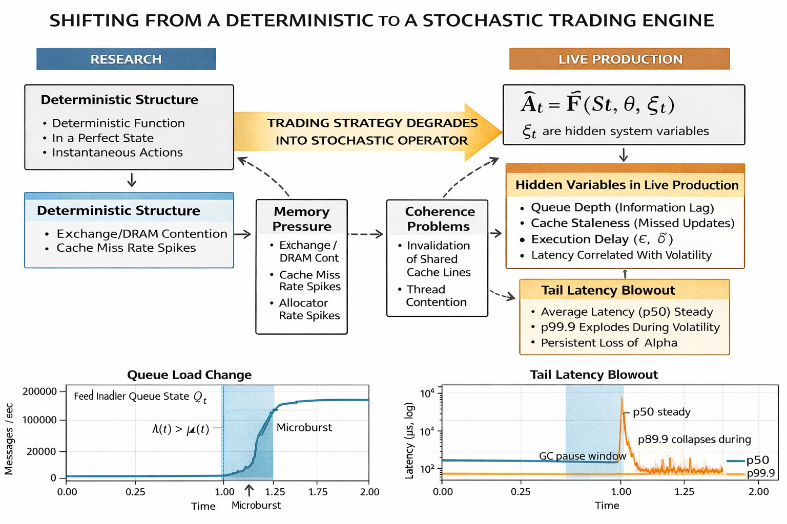
When a trading engine moves from a controlled research environment to live production, the mathematical definition of its operation changes fundamentally.
In research, the strategy is modeled as a deterministic function F:
Where At is the action at time t, St is the market state, and θ are parameters. In this environment, St is perfect, and At is instantaneous.
In production, the strategy degrades into a stochastic operator F̂:
Here, 𝜉t represents hidden system variables that act as noise terms:
Queue depth (Qt): The backlog of unprocessed messages, which acts as a proxy for the information gap between the exchange and the CPU.
Cache residency: The probability that the relevant state St is in L1/L2 cache versus main memory (RAM), introducing a variance of ~200 cycles vs ~300 nanoseconds per access.
Coherence traffic: The latency penalty induced by other cores invalidating shared cache lines, often caused by the OS scheduler or noisy neighbor threads.
Parsing jitter: The variance in time required to decode the wire format, often depending on the specific template ID or message schema variability.
The dominant risk is not that the system is slow in a linear sense. The risk is that ε (staleness) and 𝛿 (execution delay) are correlated with market volatility.
If Cov(ε, | ΔPt} > 0, your system is statistically most likely to be acting on stale data exactly when the price is moving the most. For example, during a sudden liquidity collapse, the incoming message rate spikes, increasing ε. Simultaneously, |ΔPt| is large. Your strategy might try to hit a bid that vanished 50 microseconds ago because it is still processing the queue from 100 microseconds ago. This converts what looks like technical edge into noise, effectively randomizing the PnL of the strategy. The decision function is no longer deterministic, it is a random variable dependent on the micro-state of the hardware.
The event that exposes this fragility is the microburst.
Standard Poisson arrival models fail to capture the reality of market data, which is characterized by self-similarity, heavy tails, and clustering. A microburst is is a phase transition in the queuing system (a very short, intense spike in activity).
As visualized in our queue topology simulation (plot 1 below), when arrival intensity λ(t) momentarily exceeds service rate μ(t), the queue length Qt does not just increase linearly; it undergoes a regime shift. The system transitions from a real-time state (Q≈0), where the CPU is waiting for network packets, to a batch state (Q≫0), where the network card is buffering packets faster than the PCI bus or the CPU can ingest them.
Crucially, in this batch state, the system is partially ordered. Because different components of a trading system (feed handlers, strategy logic, execution gateways, risk checks) often run on decoupled threads or separate cores, a burst desynchronizes their views of the world:
The feed handler receives update U1, U2, U3.
The strategy calculates a signal based on U1.
The risk/order manager checks limits based on U3 (because it processes a different stream or shares a flag updated asynchronously).
At this moment, the system has no single time. The strategy logic and the execution logic occupy different temporal frames. This is the main problem: The burst breaks the semantic integrity of the engine. The system is a collection of race conditions executing in parallel, where the winner is determined by cache arbitration rather than financial logic.

We must shift our perspective on what a low-latency data structure actually is.
In standard quant dev, a data structure is defined by its asymptotic complexity (O(1) lookup, O(log N) insertion). In low latency architectures, this view is insufficient because constants matter, and the cost of the worst-case operation dominates the PnL profile.
A data structure must be seen as a set of rules. It is a boundary definition that governs:
Visibility: When exactly does a write by the feed handler become visible to the strategy thread? Is it after a memory fence? Is it relaxed?
Atomicity: Can the strategy see a torn price (e.g., a bid from time t and an ask from time t+1)? If so, the strategy might compute a phantom arbitrage opportunity that exists only in the corrupted memory state.
Backpressure: How does the structure communicate to the upstream socket that it is full? Does it block? Does it drop? Does it signal the sender to slow down (which is impossible with UDP multicast)?
Lifecycle: How is the data persisted for replay without blocking the read/write path? Can we reconstruct the exact sequence of memory states from the log files?
This is different from optimizing code for instruction count. In this point we are optimizing the conditional law of decision latency. We are engineering the system such that the latency distribution P(Lt > x) decays super-exponentially, ensuring that even in the 99.99th percentile of events (the burst), the system remains within the coherence window of the market.
The implementation of this approach faces severe structural obstacles that cannot be solved by simply writing faster code:
Boundedness vs. blindness:
Infinite or dynamically resizing buffers (like
std::vectoror Python lists) hide overload. They allow the system to ingest a burst it cannot process, creating a standing wave of latency that persists long after the burst ends. The system continues to process old data while the market has moved on.
We need buffers that are strictly bounded. However, bounding a buffer requires a policy for rejection (drop vs. overwrite). This forces the strategy to handle gaps in data. A gap in a price series creates a discontinuity in derivative calculations, complicating the quant logic and requiring robust exception handling in the math itself.
Observation vs. perturbation:
Measuring latency typically involves getting timestamps (
rdtscorclock_gettime) and logging them. Writing to a log file involves blocking I/O; writing to memory involves cache pollution. The act of measuring the tail often causes the tail by evicting critical strategy data from the L1 cache to make room for telemetry structs.We need telemetry that is zero-cost in the cache-hot path, storing only summary statistics (quantiles) rather than raw logs, without allocating memory or contending for lock resources.
Consistency vs. contention:
To ensure the strategy sees a consistent snapshot (e.g., best bid and best ask from the same packet), the naive solution is a
mutexorrwlock. Locks induce context switches, force the OS to schedule threads, and stall the CPU pipeline. In a microsecond environment, a context switch is a massive penalty.We need a wait-free snapshot mechanism that guarantees consistency without blocking the writer, even if it requires the reader to retry. We trade CPU cycles (retries) for latency stability (no blocking).
Replay fidelity:
Production systems often differ from backtests because the production system has state (sequence numbers, partial fills, TCP retransmits) that the backtest ignores. A strategy that worked in the simulator fails in production because the simulator did not model the sequence of partial updates caused by network fragmentation.
We need a data structure layout that supports deterministic replay. We must be able to feed the raw wire capture into the engine and produce the exact same state transitions, bit-for-bit, as occurred in live trading. This requires treating the entire engine as a deterministic finite state machine derived solely from the input log.
This sets the stage for building a deterministic state machine capable of surviving the hostile environment of live market microstructure.
Lifecycle engineering for low latency data structures
This type of engine rests on seven pillars. These pillars are are the axioms that prevent a system from becoming non-deterministic. To continue with the previous articles, we will proceed with the examples implemented in Python.
Point 1 — Capacity-constrained processing
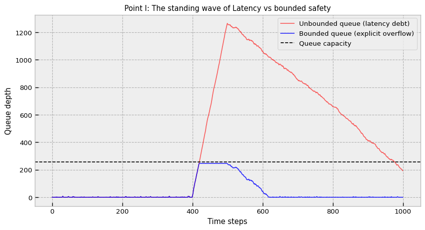
The first misconception to dismantle is the idea that larger buffers equal greater safety. In latency-sensitive systems, buffers are debt. They convert instantaneous overload (a bandwidth problem) into delayed decision error (a latency problem).
Let arrivals be a clustered process with intensity λ(t) and service rate μ(t). If we use a dynamically resizing queue (like a Python list or C++ std::vector), we implicitly allow queue length Qt ↦ ∞.
During a burst, Qt grows. If the burst lasts 100ms and the system lags by 50ms, the strategy calculates signals based on prices that are 50ms old. This is an eternity, the alpha has decayed to zero or reversed. Furthermore, the very act of resizing a dynamic container during a burst exacerbates the problem. When a std::vector or dynamic list hits capacity, the runtime must allocate a larger block of memory, copy all existing elements to the new block, and free the old one. This operation causes a massive latency spike exactly when the system can least afford it, effectively pausing processing while the queue is flooding.
The solution involves bounded and pre-assigned queues with explicit overflow. So we must use fixed-capacity, circular buffers. The overflow behavior must be defined. This forces the engineering team to confront the reality of finite resources before the market does it for them.
Drop newest: Ignore the new packet (good for keeping the strategy processing contiguous history, bad for recency). This effectively sheds load at the gateway, ensuring the internal engine never processes data faster than it can consume, but it risks blindness to the current market state.
Drop oldest: Overwrite the tail (maximizes recency, but introduces data gaps). This is equivalent to saying, “If I can’t process everything, I will at least process the most current thing.” It breaks the assumption of a continuous time series, forcing the strategy to be robust against missing ticks.
For algorithmic trading, drop oldest (circular overwrite) is often preferred for market data (we care about the now price), while drop newest might be preferred for order entry (we don’t want to skip a sequence number).
We use a numpy based Structure of Arrays. This ensures that reading a specific field (e.g., all timestamps) utilizes full cache lines, unlike an Array of Structures or a list of objects. By keeping data contiguous in memory, we minimize the CPU’s need to fetch data from main RAM, keeping the hot path executing almost entirely within L1 or L2 cache.
import numpy as np

class BoundedEventQueue:
    """
    Preallocated circular queue for fixed-schema events.
    Overflow is explicit. No GC. No resizing.
    Uses Structure of Arrays (SoA) to maximize cache locality for column-based analysis.
    """
    __slots__ = ("cap", "mask", "write", "read",
                 "ts", "typ", "sym", "px", "qty",
                 "overflow_count")

    DROP_NEWEST = 0
    DROP_OLDEST = 1

    def __init__(self, cap_pow2: int):
        # Enforcing power of 2 allows bitwise AND masking (x & mask)
        # which is significantly faster than modulo (x % cap) and avoids division instructions.
        if cap_pow2 & (cap_pow2 - 1) != 0:
            raise ValueError("Capacity must be a power of 2.")
        self.cap = int(cap_pow2)
        self.mask = self.cap - 1
        self.write = 0
        self.read = 0

        # Fixed schema (SoA) - Preallocation prevents runtime allocation
        # We assume 64-bit timestamps and 32-bit prices/quantities.
        self.ts  = np.empty(self.cap, dtype=np.uint64)
        self.typ = np.empty(self.cap, dtype=np.uint8)
        self.sym = np.empty(self.cap, dtype=np.uint16)
        self.px  = np.empty(self.cap, dtype=np.int32)
        self.qty = np.empty(self.cap, dtype=np.int32)

        self.overflow_count = 0

    def push(self, ts, typ, sym, px, qty, overflow_policy=DROP_OLDEST) -> bool:
        """
        Push operation that is strictly O(1) and allocation-free.
        """
        # Check occupancy
        size = self.write - self.read
        if size >= self.cap:
            self.overflow_count += 1
            if overflow_policy == self.DROP_NEWEST:
                return False
            # DROP_OLDEST: We forcibly advance the read pointer, effectively
            # "forgetting" the oldest unread message to make space for the new one.
            # This maintains the "freshness" of the buffer at the cost of history.
            self.read += 1

        # Bitwise mask for circular wrapping
        i = self.write & self.mask

        # Direct memory access without object overhead
        self.ts[i]  = ts
        self.typ[i] = typ
        self.sym[i] = sym
        self.px[i]  = px
        self.qty[i] = qty

        self.write += 1
        return True
Note: Full low latency data structures is in the provided code of the appendix.
This structure forces the architect to answer the question: What happens when overflow_count > 0? The answer usually involves entering a risk reduction mode. If the queue overflows, the strategy is legally blind; the only safe action is to widen quotes or pull orders until the overflow_count stabilizes and the system catches up.
Point 2 — Tail telemetry
The second pillar is observability. You can’t manage what you can’t measure, but measuring the 99.9th percentile (Q0.999) of latency is statistically difficult.
A naive average (mean) is useless in HFT because latency distributions are heavy-tailed (Power Law or Pareto-like). A slow event might be 1000x slower than the median due to an OS context switch, a minor page fault, or a Garbage Collection pause. In these distributions, the mean is a misleading artifact of the tail.
The standard approach of storing all latency samples to compute an exact quantile is memory-prohibitive and causes cache pollution. Writing every single latency sample to a log file acts as an observer effect—the I/O overhead of logging the latency creates the latency you are trying to measure. We need a streaming quantile estimator—an algorithm that updates the estimate of the tail using constant memory.
The P2 (piecewise-parabolic) algorithm is ideal here. It maintains 5 marker points that track the shape of the CDF around the target quantile. As data streams in, these markers adjust their height and position to approximate the curve, allowing for accurate tail estimation without ever storing the raw data points.
This matters because if your telemetry system allocates memory (e.g., creating a string for a log message logger.info(f"Latency: {lat}")), that allocation itself can trigger a Garbage Collection pause or a malloc lock, causing the very latency spike you are trying to record. Zero-allocation telemetry is a requirement, not an optimization.
import numpy as np

class P2Quantile:
    """
    Streaming quantile estimator using P^2 algorithm.
    Memory usage: Fixed (small arrays).
    Allocations per update: Zero.
    """
    def __init__(self, p: float):
        self.p = p
        # Markers for the P^2 algorithm
        # We only need 5 doubles to track the curve shape.
        self.q = np.zeros(5, dtype=np.float64)
        # ... (initialization logic omitted for brevity) ...

    def update(self, x: float):
        # Complex logic to adjust markers based on parabolic interpolation.
        # This allows us to estimate the 99.9th percentile with high accuracy
        # after observing N samples, without storing N samples.
        # This function must be allocation-free to run in the hot path.
        pass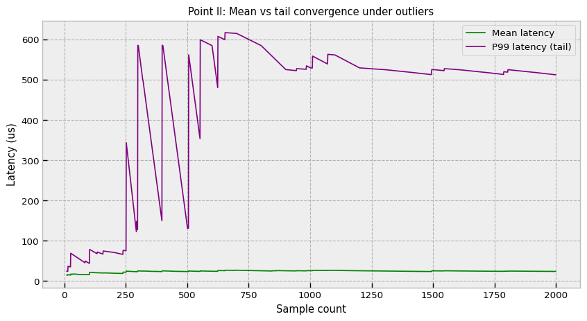
The output of this estimator should be fed directly into the autotrader’s logic. If Q0.999 > Threshold, the strategy should automatically widen spreads or reduce size, acknowledging that its reaction time has degraded. This turns telemetry from a passive debugging tool into an active risk control.
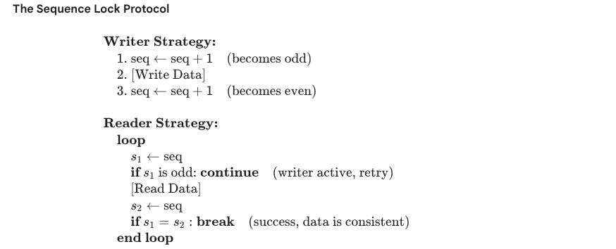
Point 3 — Consistency domains without global locks
The third pillar addresses the torn read problem.
Imagine a book update arrives:
Bid Price: 100.05
Ask Price: 100.07
The strategy thread reads the Bid (100.05). Before it reads the Ask, a new update arrives:
Bid Price: 100.06
Ask Price: 100.08
If the strategy reads the new Ask (100.08) combined with the old Bid (100.05), it sees a spread of 0.03 (100.08 - 100.05). But the real spread was always 0.02. If the strategy’s logic is “Buy if spread > 0.025”, this phantom spread triggers a trade that immediately loses money. This is a Heisenbug that disappears when you add logging (because logging slows the writer down enough to avoid the race).
To prevent this without locking the writer (which stalls the feed handler), we use a Sequence Lock (Seqlock). A standard Mutex would force the writer to wait for readers, which is unacceptable for a feed handler that must process millions of messages per second.
from multiprocessing import Value
import ctypes

class SharedSnapshot:
    def write(self, values):
        s = self.seq.value + 1
        self.seq.value = s       # Odd = Locked / Dirty
        # Implicit memory barrier needed here in C++ (std::memory_order_release)
        self.arr[:] = values     # Bulk copy
        # Implicit memory barrier needed here in C++ (std::memory_order_release)
        self.seq.value = s + 1   # Even = Unlocked / Clean

    def read(self, out):
        s1 = self.seq.value
        if s1 & 1: return False  # Collision: Writer is currently writing

        # Optimistic read: assume no one is writing
        out[:] = self.arr

        s2 = self.seq.value
        # If s1 != s2, it means the writer started writing while we were reading.
        # The snapshot in 'out' is corrupted.
        return s1 == s2          # Verification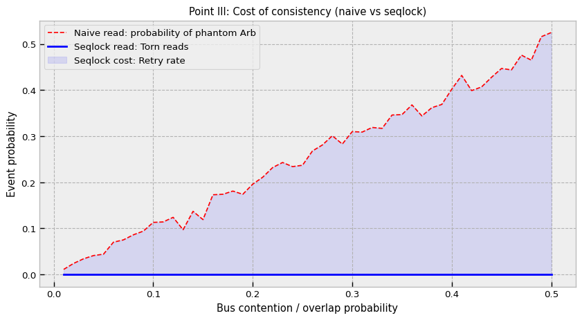
This defines a consistency domain. All fields inside arr are guaranteed to be from the same logical timestamp if read() returns True. This effectively eliminates a class of synchronization errors where the strategy acts on state combinations that never existed in reality. It shifts the cost of concurrency from the writer (who must never block) to the reader (who must occasionally retry), which aligns perfectly with the priorities of a trading system.

Point 4 — Schema and layout hashing
In a dynamic language like Python (often used for the strategy layer wrapping C++ cores), or even in C++ with extensive templating, the physical layout of data can shift silently between code versions. This schema drift is often invisible in source code but fatal in the CPU cache.
Consider a developer who adds a single bool flag to an order struct to track a new risk check.
Before: The struct was 16 bytes (aligned). It fits perfectly 4 times into a standard 64-byte CPU cache line.
After: The struct is nominally 17 bytes.
However, the compiler or interpreter will not allocate exactly 17 bytes. To maintain memory alignment requirements for the CPU, it will likely add padding bytes, swelling the size to 24 or 32 bytes. This seemingly trivial change has hardware implications. It reduces the number of items that fit in a CPU cache line, increasing the cache miss rate during iteration. Furthermore, a 65-byte object (just 1 byte over the line) requires two cache line fetches to read a single object, effectively doubling the memory bandwidth cost for that access pattern.
Additionally, if the strategy logic relies on structured arrays or memory mapping, a mismatch in dtype definitions between the C++ writer and the Python reader can cause the runtime to perform an implicit copy-cast during data access. Instead of a zero-copy view, the system silently mallocs new memory and copies the data to fit the expected layout, introducing microsecond-level stalls on every access.
The solution is known as schema hashing. We treat the memory layout as a strict API. At startup, the system computes a hash of the data type’s internal memory layout (offsets, item sizes, field types). This hash acts as a cryptographic signature of the physical memory contract.
import numpy as np
import hashlib

def dtype_layout_hash(dt: np.dtype) -> str:
    """
    Computes a hash of the physical layout of a numpy dtype.
    Includes byte offsets, field order, and alignment details.
    """
    dt = np.dtype(dt)
    # Capture critical layout details that affect binary compatibility
    parts = [f"itemsize={dt.itemsize}", f"aligned={dt.isalignedstruct}"]
    for name in dt.names or ():
        f, off = dt.fields[name][0], dt.fields[name][1]
        parts.append(f"{name}:{f.str}@{off}")

    # Create a unique signature for this layout
    payload = "|".join(parts).encode("utf-8")
    return hashlib.sha256(payload).hexdigest()[:16]

# If this hash changes between the Writer (Feed Handler) and Reader (Strategy),
# the system refuses to start, preventing silent data corruption or performance degradation.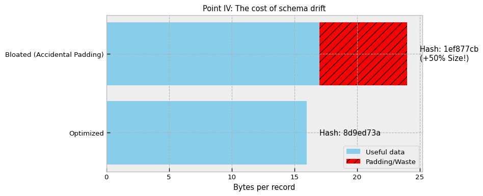
This enforcement prevents release drift, where performance degrades slowly over time due to minor schema bloating, ensuring that the cache locality you engineered in Version 1.0 remains intact in Version 10.0.
Point 5 — Deterministic replay