


Table of contents:
Introduction.
The conflict between research and production.
Micro-machines architecture.
Design point 1: Cache-line.
Design point 2: Coherence engineering.
Design point 3: Topology-aware state.
Design point 4: Page-level engineering.
Design point 5: Control-flow predictability.
Design point 6: Wire-format and parsing structures.
Design point 7: Time and numeric representation.
Before you begin, remember that you have an index with the newsletter content organized by clicking on “Read the newsletter index” in this image.

Introduction
Most performance debates in trading start at the wrong layer. Quants argue about languages, compilers, and fast code, as if latency were a property of instructions. In production, latency is a property of structure: how state is laid out, how it is shared, how often the machine is forced to translate addresses, and how predictable the control flow remains. The micro-pauses that ruin fills are concrete events.
The real conflict is that research optimizes for average throughput, while production lives under the question: did the system took the decision before the market boundary moved?
That boundary compresses exactly when volatility rises—precisely when your edge is largest and the penalty for being late is most asymmetric. This is why mean latency is a comforting metric and a dangerous one: the tail determines whether cancels land, hedges actually hedge, and risk gates engage on time.
Most systems fail here because their data structures are designed for convenience, not for invariants. Pointer-heavy graphs, heterogeneous containers, dynamic dispatch, and ad-hoc parsing become regime-dependent under load. The result is a bimodal latency distribution: stable in calm sessions, unstable when message rates spike.
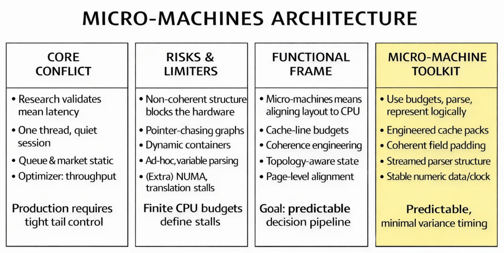
The solution is to design micro-machines architectures: treat the CPU as a collection of finite budgets rather than a generic processor. There is a cache-line budget (useful bytes per fetch), a coherence budget (how often lines can bounce between cores), a translation budget (distinct pages touched per unit time), and a prediction budget (branch stability). When you exceed these budgets, the penalties arrive as discontinuities that dominate p99 behavior, not as smooth slowdowns that averages can summarize.
If you want to go deeper in this topic, check this PDF:
The design points that follow are for stability constraints: engineer cache-line layouts to keep hot fields hot, engineer coherence to prevent false sharing and line bouncing, make state topology-aware to avoid NUMA randomness, engineer at the page level to keep translation predictable, stabilize control flow with table-driven state transitions, parse with rigid wire formats that don’t allocate or branch unpredictably, and use deterministic time and numeric representations to eliminate threshold drift. The target is a tighter distribution so the engine you deploy is the engine you validated.
The conflict between research and production
In the research phase, a pipeline is evaluated primarily by mathematical correctness and average throughput. We treat the compute substrate as deterministic. But in live production, the objective function collapses to a binary state: did you express the decision before the market boundary shifted?
This boundary is not static. It is a dynamic variable that compresses aggressively during volatility bursts—precisely the regime where your edge is highest. The dilemma is effectively a race against a shrinking liquidity window.
Most traders accept this premise theoretically, yet define their systems with convenient structures—pointer-heavy graphs, dynamic dispatch, and heterogeneous containers—that practically guarantee failure. The result is a system with a bimodal latency distribution.
In the Asian session (quiet regimes), the workflow fits within the window. However, during the London session or when this session overlaps with the American session, state consistency degrades, branch predictors go astray, the CPU gets stuck on page traversals, and cache misses occur. Sometimes, you even experience micro-pauses that disappear in the average statistics but manifest as failed data fills.
This is not due to a problem with the code or the interpreter, but rather a structural mismatch between the data design and the hardware you are using.
As you already know, a live trading model is a composition of a signal and a timing apparatus. If the timing apparatus behaves stochastically under load, the realized model differs from the validated one. This divergence manifests in four specific failure modes:
State incoherence under concurrency means risk flags or inventory states may be consistent within one thread but stale in another at the moment of decision.
Service time variance explodes as the compute work per message becomes regime-dependent due to cache misses or coherence traffic.
Latency amplification occurs where small increases in mean service time produce non-linear increases in p99 latency as utilization approaches saturation.
Numerical representation drift in float-heavy state machines creates rounding artifacts that lead to inconsistent thresholds around cancel/replace boundaries.
These issues are not resolved by faster code but by selecting data layouts that behave predictably on specific hardware.
The failure that necessitates this architectural shift is rarely a crazy outage but a repeating small incident. For example, a hedge engine receives a burst and computes a cancel/replace based on a risk condition that was true when reading one field but false when reading another. The system sends the wrong intent, and the market punishes the strategy via adverse selection. While post-mortems often debate signals or slippage models, the conflict is that the internal data structure did not provide atomicity at the semantic level required by the strategy. The alpha survived, the code executed, but the structure of state rendered the decision non-deterministic.

Micro-machines architecture
The next step in latency engineering is accepting that the microarchitecture often behaves adversarially because data layouts provide it no alternative. A senior quant must view the CPU as a collection of finite budgets rather than a generic processor. These include the cache line budget (managed at 64-byte granularity), the coherence budget (the frequency of forced invalidations), the translation budget (distinct pages touched per unit time), and the prediction budget (stability of branches) . These budgets are concrete; when exceeded, they manifest as measurable stalls.
Addressing these budgets involves overcoming practical obstacles:
Averages deceive: a 10% improvement in mean compute time is irrelevant if the tail is driven by coherence or translation events.
Concurrency changes everything: a single-core benchmark that performs well can become unstable when the pipeline is split across cores.
State is not scalar: it is a set of fields that must be read and written with a semantic consistency boundary.
Finally, the dynamic nature of Python, while convenient, poses a significant danger in the hot path. The challenge is to build structures that enforce predictability even when the flow rate changes abruptly.
Design point 1: Cache-line
A common misconception is that contiguous memory guarantees speed. While contiguity is necessary, it is insufficient. If fields straddle cache lines or structures force split loads, the system can remain contiguous yet suffer unpredictable behavior. In trading, this risk is acute because order state is accessed under stress. If a hot field, such as best_bid_px, shares a cache line with a cold field, like client_tag, accessing the cold data drags the line into the cache, evicting necessary data and creating churn that manifests as jitter.
Cache lines are fetched as a unit, typically 64 bytes. Two mechanisms degrade performance: split accesses, where a load crosses a line boundary requiring two fills, and line pollution, where cold fields waste cache capacity. We model the cost of reading a field x as:
Here, I(x) indicates a cache miss and J(x) indicates a split access. The variance of C(x) is driven by the Bernoulli events I(x) and J(x) rather than the baseline cost C0. The engineering objective is to drive P(I=1) and P(J=1) toward zero in the hot path.
One cannot force L1 residency from Python, but one can enforce alignment and separation. The first step is an alignment audit to ensure arrays begin at stable offsets relative to cache lines.
import numpy as np
CACHELINE = 64

def addr_mod_cacheline(arr: np.ndarray) -> int:
    return arr.ctypes.data % CACHELINE

# Packed vs Aligned Dtypes
packed = np.dtype([('px', 'f8'), ('qty', 'f4'), ('ts', 'u8'), ('tag', 'u8')], align=False)
aligned = np.dtype([('px', 'f8'), ('qty', 'f4'), ('ts', 'u8'), ('tag', 'u8')], align=True)

A = np.zeros(1024, dtype=packed)
B = np.zeros(1024, dtype=aligned)
print('packed addr%64:', addr_mod_cacheline(A))
print('aligned addr%64:', addr_mod_cacheline(B))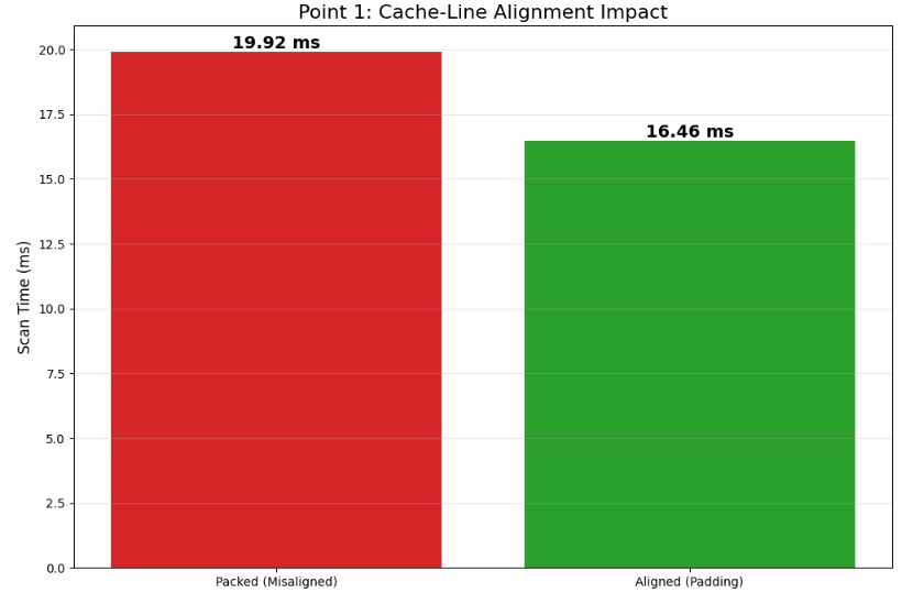
The structural solution involves separating hot and cold fields into distinct arrays keyed by the same index, ensuring that access patterns remain predictable and cache lines are populated only with relevant data.
N = 1024 # random chosen for this example

# HOT: fields used on every message
hot_px = np.empty(N, dtype=np.float64)
hot_qty = np.empty(N, dtype=np.float32)
hot_ts = np.empty(N, dtype=np.uint64)

# COLD: metadata rarely used in hot path
cold_tag = np.empty(N, dtype=np.uint64)
cold_flags = np.empty(N, dtype=np.uint32)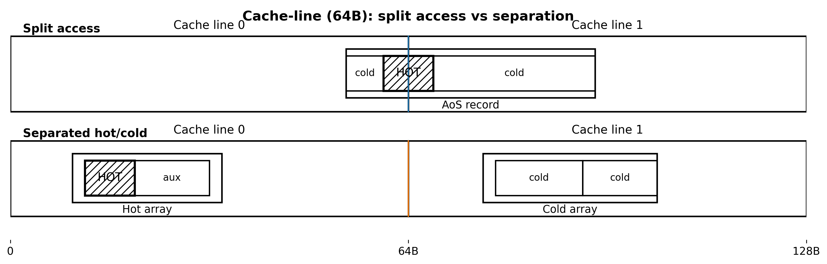
By enforcing alignment and segregating hot/cold fields, we minimize local stalls and maximize the density of useful data per fetch .
Design point 2: Coherence engineering
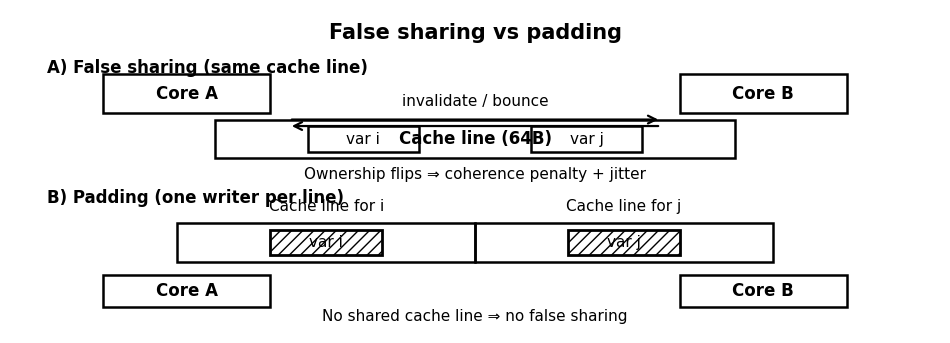
The belief that splitting work across cores inevitably lowers latency is dangerous. Multi-core performance is not additive when state forces coherence traffic. Worst-case coherence patterns appear in critical paths: per-symbol risk flags, shared order state, and global counters. If two cores write to different variables that share a cache line, false sharing occurs, causing the line to bounce between cores despite the data being logically independent.
Best protocols maintain a single writer for each line. If Core A writes to a line and Core B writes to a different word on the same line, the line invalidates repeatedly. This produces a latency term Tcoh≈nbounces × tinvalidate, where nbounces scales with the event rate.
We treat service time per message as S=S0+B, where B is the coherence penalty. If bounces occur as a Poisson process with rate ν and cost τ, then:
This variance is critical because queueing tail behavior is highly sensitive to service time variance. As utilization ρ→1, waiting time quantiles explode non-linearly.
To avoid false sharing without complex lock-free structures, we use padding. Each worker’s counter must occupy its own cache line.
import numpy as np
CACHELINE = 64
PAD_WORDS = CACHELINE // 8
n_workers = 8

# One uint64 counter per worker, padded to one cache line each
counters = np.zeros(n_workers * PAD_WORDS, dtype=np.uint64)

def counter_view(i: int) -> np.ndarray:
    return counters[i * PAD_WORDS : (i+1) * PAD_WORDS]

# Worker i increments without touching Worker j's cache line
counter_view(3)[0] += 1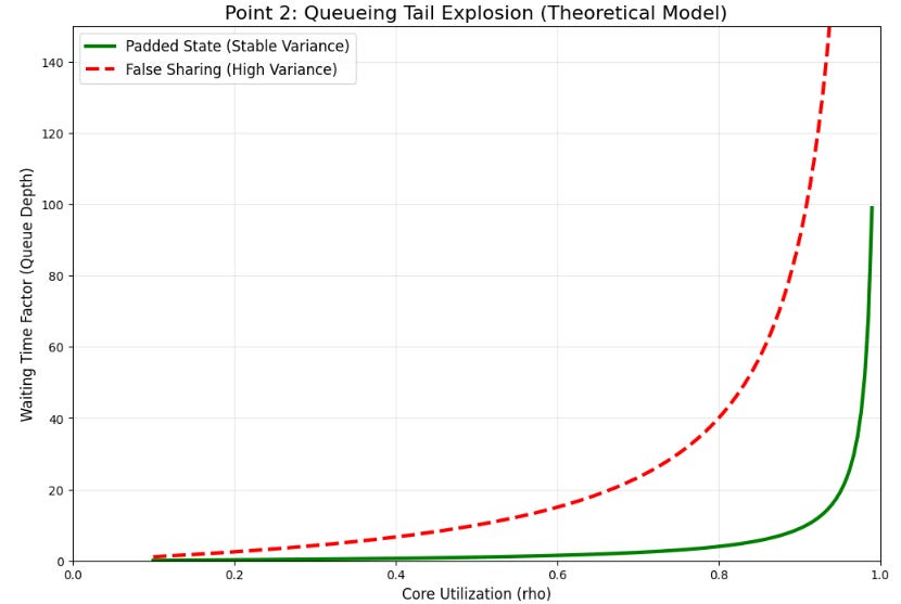
For global metrics like inventory, we avoid updating a global scalar from multiple workers. Instead, we maintain per-shard state and reduce it only on demand or on a schedule, decoupling the write frequency from the read frequency .
Design point 3: Topology-aware state
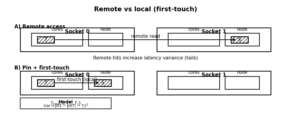
It is a misconception that memory is uniform; on multi-socket machines, memory access possesses locality. Allocating state on one node and reading it from another incurs a penalty that is regime-dependent. This risk appears in large symbol universes or multi-process architectures where processes are pinned to different sockets . In calm markets, cross-node penalties are masked, but in bursts, they become part of the tail.
A NUMA miss changes effective bandwidth and increases variance. We model access time as:
If the probability of remote access p changes with thread scheduling, Tmem becomes stochastic. The variance is given by:
This variance again feeds into queueing tails.
Since the OS kernel typically uses a first touch policy—where the node that first writes to a page owns it—we must ensure the consumer process initializes the state.
import numpy as np
import os

def allocate_and_touch(shape, dtype, touch_value=0):
    x = np.empty(shape, dtype=dtype)
    x[...] = touch_value  # Touch all pages by writing
    return x

def pin_to_cores(cores):
    os.sched_setaffinity(0, set(cores))

# Pin to cores [0,1,2,3] and then allocate state locally
pin_to_cores([0,1,2,3])
state = allocate_and_touch((10000,), np.float64)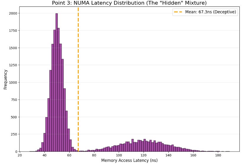
As you see, pinning is much more than performance optimization; indeed, it is a stability mechanism that reduces the randomness in execution location, eliminating a hidden mixture component in the latency distribution.
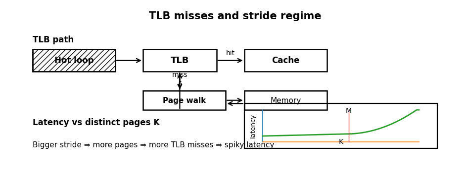
Design point 4: Page-level engineering
Another pervasive misconception in low-latency systems is that cache misses represent the primary memory bottleneck. In reality, caches are only half the story; before the CPU can fetch a cache line, it must translate the virtual address to a physical address via the Translation Lookaside Buffer (TLB) . If a strategy touches too many pages too quickly, the TLB misses, and the hardware page walker intervenes, stalling the pipeline.
This risk is acute when scanning large state arrays with poor stride patterns or maintaining sparse per-symbol objects spread across the heap . A classic pathology involves a hot loop that reads just a few bytes from a vast number of pages; while the data cache sees a low volume of bytes, the TLB sees an overwhelming number of distinct pages.
We model the translation cost as a variance injection term:
where δ is the penalty of a page walk and p(K) is the probability of a miss given K pages touched per message. As K exceeds the TLB’s coverage capacity M, the miss rate increases sharply, causing latency to become spiky.
The impact of access patterns is quantified by approximating the number of distinct pages touched when scanning N elements of size b with stride s:
where P is the page size (typically 4KB). This relationship reveals that stride is a multiplier for page footprint. A stride that forces jumps across page boundaries can turn a computationally trivial loop into a translation nightmare.
We can diagnose this regime change qualitatively by measuring scan latency as a function of stride. The following Python snippet shows the non-linear latency jump that occurs when the stride causes page thrashing:
import numpy as np
import time

def scan_sum(arr: np.ndarray, step: int) -> float:
    t0 = time.perf_counter_ns()
    s = float(arr[::step].sum())
    t1 = time.perf_counter_ns()
    return (t1 - t0) / 1e6  # ms

N = 50000000
arr = np.ones(N, dtype=np.float64)
# Observe regime change as step size increases
for step in [1, 2, 4, 8, 64, 512, 4096]:
    print(step, scan_sum(arr, step))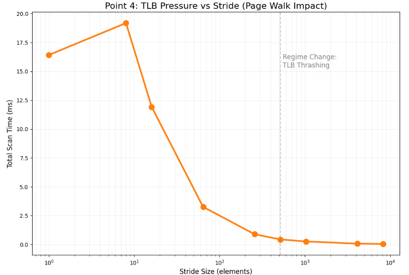
The engineering response is to keep hot loops page-local by operating on contiguous blocks and avoiding sparse pointer chasing. Where appropriate, utilizing huge pages can increase effective coverage, though this requires OS support and careful operational discipline.

Design point 5: Control-flow predictability