


Table of contents:
Introduction.
Do we really need low-Latency data structures?
Risk and limitations of the data structures.
Low latency, reframed: Risk distribution.
Memory and allocation.
Core optimization.
Tail-latency budgeting as a first-class risk metric (quantile engineering).
State and flag encoding under memory-bandwidth constraints.
SoA vs AoS for feature pipelines.
Preallocation and out=.
Queueing primitives.
Zero-copy paths and multiprocess topologies.
Before you begin, remember that you have an index with the newsletter content organized by clicking on “Read the newsletter index” in this image.

Introduction
You can have the right signal, the right risk limits, and the right order type, and still lose money because your system expresses that decision at the wrong moment. That failure mode is especially cruel because it doesn’t look like bad alpha in a backtest; it looks like slippage, adverse selection, and fills that degrade exactly when you most need precision. The strategy survives on paper while the execution layer taxes it in production.
Most teams treat that tax as an engineering inconvenience: optimize later, refactor later, rewrite later. But latency is not a single number you improve. The market doesn’t care about your median. It cares about the rare stalls that occur during stress, when queues build, spreads widen, and your signal’s half-life collapses. Those stalls are where good research becomes a losing business.
Today we take a different stance: the execution pipeline is a risk book, and data structures are positions inside it. Each allocation, copy, branch, cache miss, and serialization step is exposure—not in dollars, but in timing error. If your system occasionally becomes unavailable for milliseconds, you are effectively holding stale orders with unpriced optionality against faster participants.
If you want to go deeper, don’t forget to check that:

So the goal here is not to make Python fast in the abstract. The goal is to make the latency profile boring: predictable under load, stable under bursts, and engineered around hard budgets. Think of it as deadline-driven execution:
A trade has value only while it arrives before a moving boundary. Past that boundary, correctness decays into noise.
What follows is a practical framework for designing that boringness: treating tail latency as a first-class risk metric, treating memory bandwidth as a scarce resource, and treating the allocator as a hazard to be removed from the hot path.
Do we really need low-Latency data structures?
In algorithmic trading, low latency is frequently fetishized as a vanity metric—a badge of honor for engineers who enjoy optimizing C++ templates, shaving nanoseconds off serialization protocols, or debating the merits of kernel bypass networking. This is an error in categorization that pervades the industry. Latency is not a stylistic preference, a marketing bullet point, or a nice-to-have feature for the roadmap; it is a measurable, deterministic property of your execution pipeline:
Market event → State update → Signal generation → Risk check → Order transmission.
Every discrete step in this chain introduces delay. More critically, every step introduces variance.
The uncomfortable dilemma facing quantitative development teams—particularly those utilizing Python for live execution—is that low latency is often treated as an optional optimization phase, something to be bolted on once the strategy demonstrates alpha.
I know what you’re going to say: Python is for prototyping and C++ is for running code. But many retailers, and even small businesses, can’t do that, due to time and cost constraints. Yes, I know, maybe they’ve done it wrong from the start, maybe they should invest more in migrating their entire infrastructure. But for whatever reason, they can’t.
So this creates a dangerous, often fatal, path dependency. Research code, optimized for vectorized throughput and batch processing (e.g., pandas DataFrames loaded from Parquet files), becomes production code. This architecture functions adequately in quiet markets where arrival rates are Poisson-distributed and manageable. But when the regime changes—a volatility spike, a venue microburst, or a specific symbol becoming the locus of global attention—the infrastructure reveals its true nature.
The senior quant’s version of this dilemma is not the binary, simplistic question “Are we fast?” It is the statistical question regarding the distribution of outcomes:
Are we optimizing Expected Latency E[L] or Tail Latency Q99.9(L)?
If you optimize for the average case (E[L]), you are implicitly accepting that in the moments of highest market stress—when the opportunity cost is highest, liquidity is most fleeting, and spreads are widening—your system will perform at its worst. This is the definition of negative convexity. If you operate strategies where the marginal expected return is a function of queue position, adverse selection avoidance, or reactive hedging, latency is not an engineering detail. It is a core parameter of the execution model. It directly impacts fill probabilities (Pfill), slippage (S), and effective spread capture.
Consider the implications of average latency in a winner-takes-all auction mechanism like a limit order book. If your system is faster than 90% of the market 90% of the time, but slower than the market during the 10% of intervals where 80% of the volume trades, your effective capture rate is near zero. You are winning races that have no prize money. Therefore, the necessity of low-latency data structures is not about speed in the abstract. It is about reducing the probability of wrong timing outcomes that invalidate the alpha model. We do not need to be fast to feel good; we need to be fast to reduce the timing error term in our PnL equation. A strategy that generates 2 bps of edge but surrenders 3 bps due to tail-latency-induced slippage during volatility is not a good strategy with bad tech; it is a losing strategy.

Risk and limitations of the data structures
The primary risk in Python-based trading systems is not the interpreter overhead itself (though that exists and sets a theoretical floor of perhaps 10-20 microseconds), but the memory access patterns dictated by standard data structures. Just use NumPy is an insufficient heuristic; in fact, naive NumPy usage can be detrimental in event-driven loops. A data structure implies a rigid contract with the hardware. It dictates:
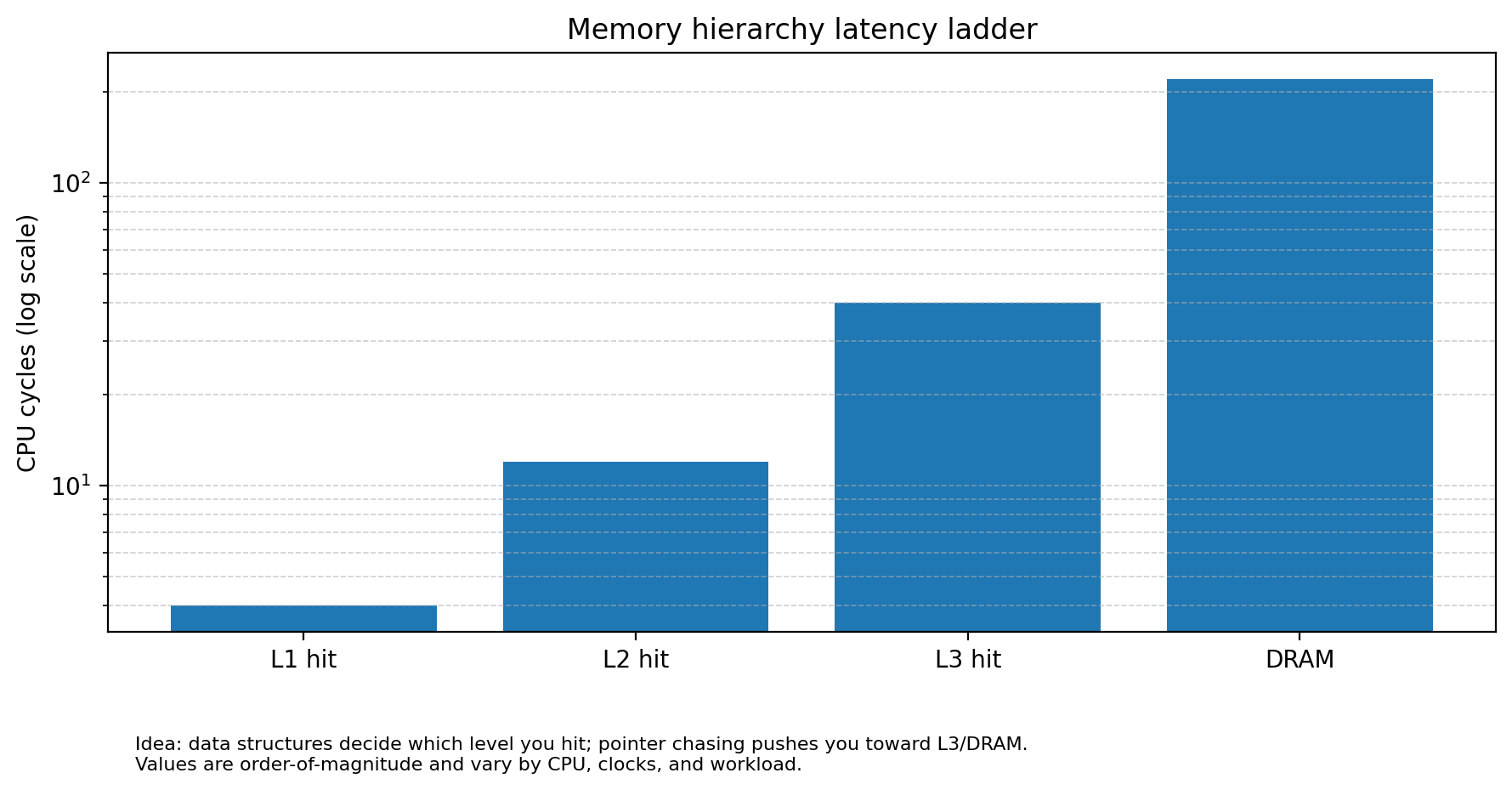
Memory access patterns: Modern CPUs depend heavily on hardware prefetchers to predict which data to load into the L1 cache before the instruction requests it. Prefetchers thrive on linearity. Are we reading contiguous blocks, or are we chasing pointers across the heap? Random access into a fragmented heap results in Cache Misses (L1/L2/L3). A single L3 cache miss can stall the CPU pipeline for 300+ cycles. If your data structure requires three pointer dereferences to read a price (e.g.,
OrderBook→Level→Price), you are guaranteeing execution stalls.
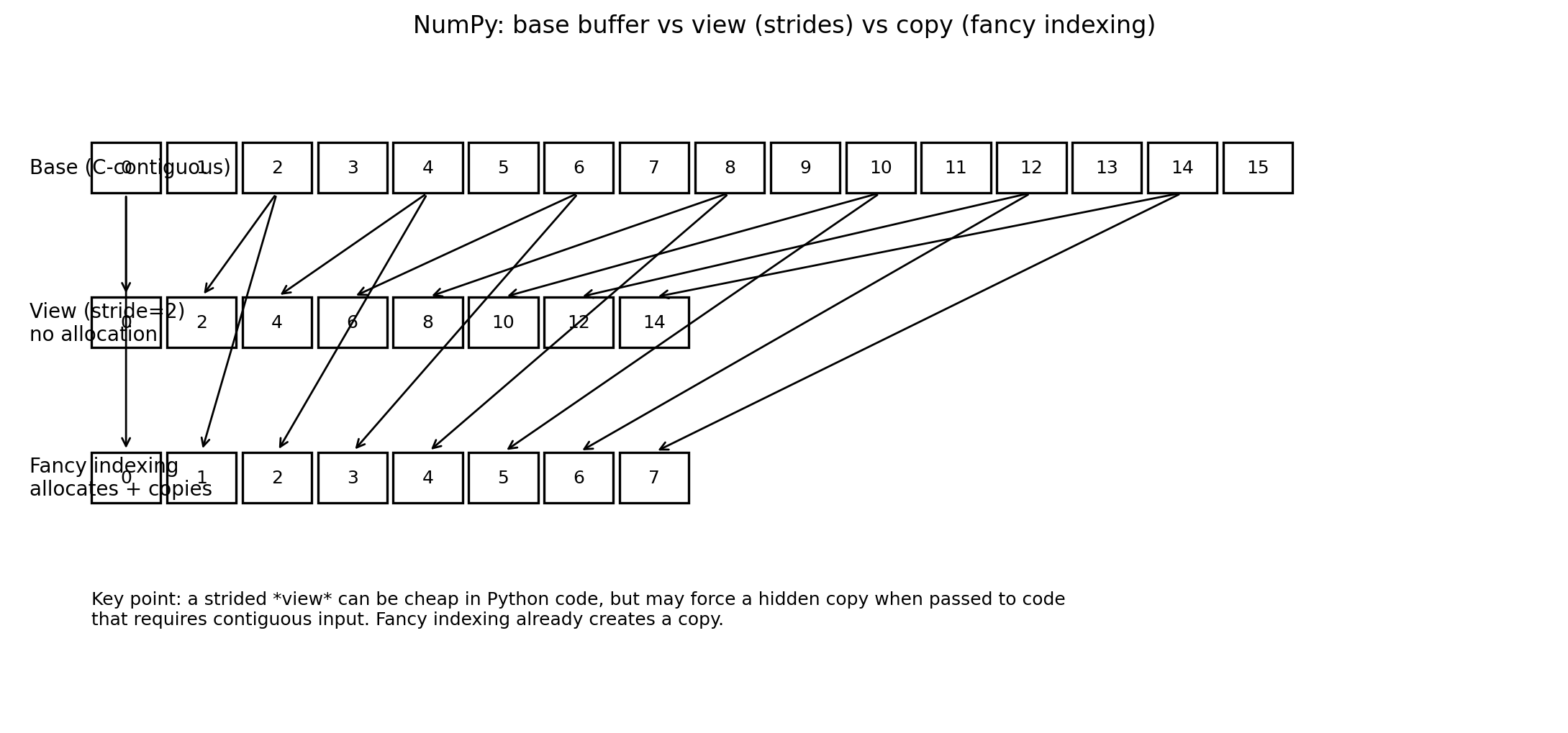
Copy semantics: Where is data duplicated? Is the copy operation visible to the developer, or hidden behind a convenient API like
fancy_indexingor slicing that triggers a deep copy? In Python, ease of use often correlates inversely with memory efficiency. For example, calling a C-compiled function that expects a C-contiguous array with a non-contiguous slice forces NumPy to silently allocate a new buffer, copy all data, execute the function, and then potentially copy results back. This is invisible in the code but devastating to the memory bus.
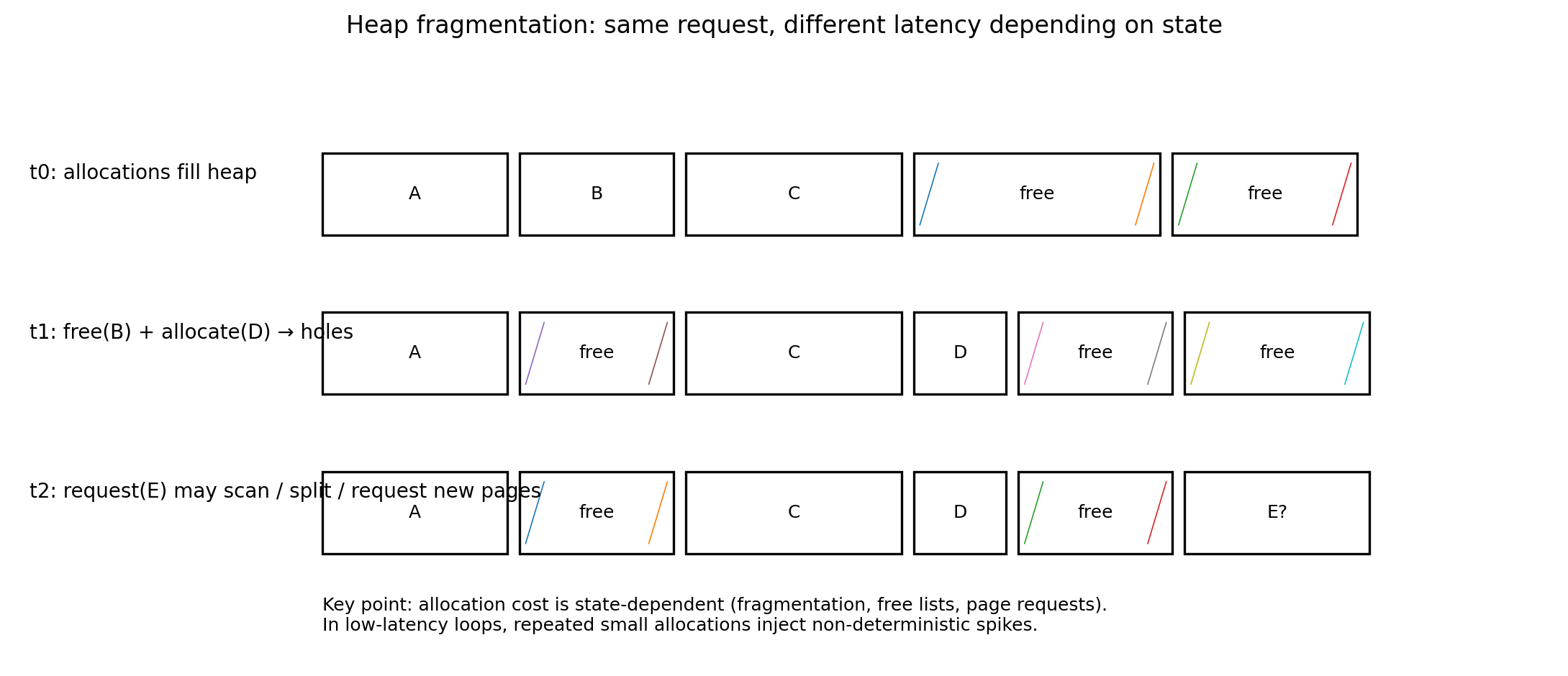
Allocation behavior: Does this operation require finding new memory pages? Does it trigger the OS allocator (
malloc/free)? Does it invoke the Python Garbage Collector? Allocation is non-deterministic; it depends on the fragmentation state of the heap at that exact moment. Requesting 64 bytes when the heap is clean might take 50ns. Requesting 64 bytes when the heap is Swiss-cheesed by fragmentation might take 5µs as the allocator searches for a contiguous block or requests new pages from the OS kernel.
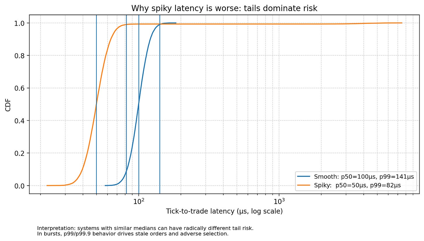
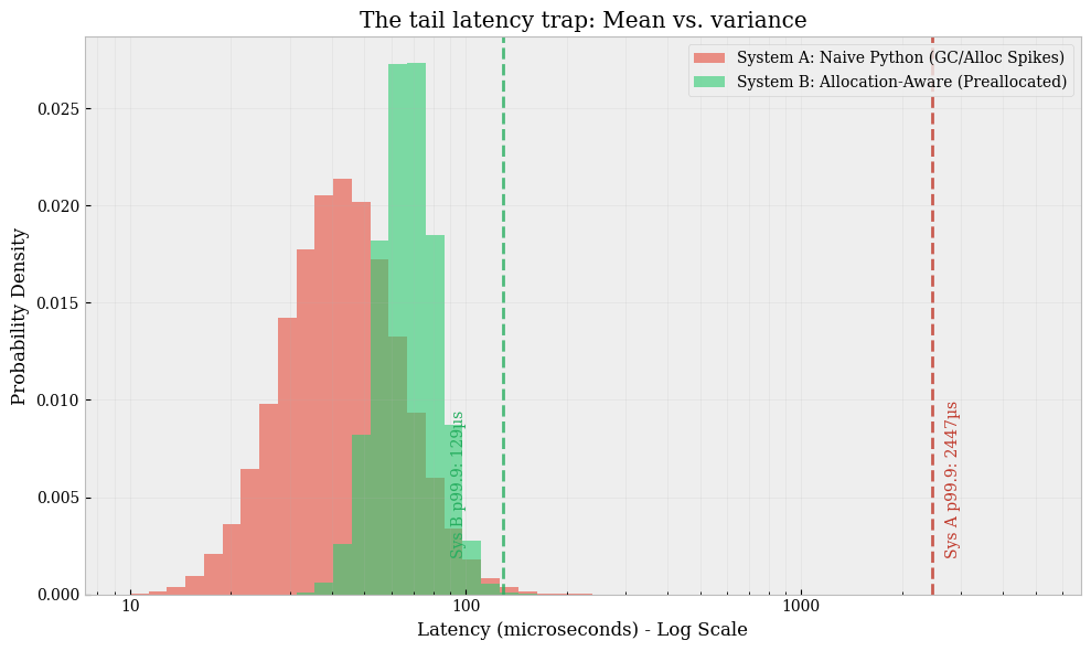
Latency distribution: Does the system exhibit consistent service times, or is it spiky? In trading, spiky latency is structurally worse than slower-but-smooth latency. A system with a median tick-to-trade time of 50μs and a p99 of 5ms is significantly more dangerous than a system with a median of 100μs and a p99 of 120μs. The former implies that during a burst, the system effectively collapses. This collapse creates stale orders resting in the book, waiting to be picked off by faster competitors who have already updated their valuation models using the new market data you haven’t processed yet.

The specific risks introduced by naive structure choices include:
Hidden copying: Implicit casting (e.g., performing arithmetic between
float32andfloat64resulting in an upcasted temporary array) ornp.ascontiguousarraycalls in hot paths. A copy operation is O(N) bandwidth consumption; doing this on every tick saturates the memory bus (DRAM bandwidth), which is often the tightest bottleneck in modern multi-core systems.Allocator jitter: Repeated temporary array creation in chained expressions (e.g.,
A = B * C + D) forces the allocator to thrash. This involves not just the time to allocate, but the time to zero-out memory for security, and the degradation of cache locality. It fragments the heap, increasing the time complexity of finding a free memory block for subsequent allocations.Bandwidth saturation: Using
np.bool_(1 byte) for binary flags wastes 8x memory bandwidth compared to bit-packed representations. In a bandwidth-constrained environment—which describes all modern HFT servers sharing Last Level Cache (LLC) across cores—wasting bandwidth is equivalent to throttling your CPU. Reading 8 bytes to get 1 bit of information is a 6300% efficiency loss.Cache thrashing: Array-of-Structures layouts (e.g., a list of
Tradeobjects) force the CPU to load cache lines containing data (e.g.,exchange_order_id,client_tag,flags) that are irrelevant to the current calculation (e.g.,mid_price). This reduces the effective cache size available for the relevant data, causing higher eviction rates. If your working set for a calculation exceeds L2 cache size because of structure bloat, your performance falls off a cliff.
The core problem here manifests during a pivotal event. Consider a mean-reversion strategy that appears stable during backtesting and low-volatility paper trading. The strategy relies on comparing the order book imbalance of a correlated ETF against the futures contract.
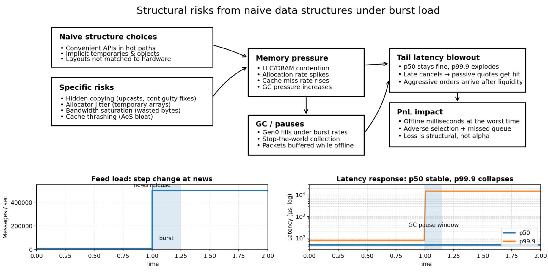
A macro news release (e.g., non-farm payrolls) triggers an auction imbalance burst. The feed handler rate jumps from a manageable 10,000 messages/sec to a torrential 500,000 messages/sec. This is not a gradual ramp; it is a step function change in load.
In this scenario, the alpha model remains valid. The signal is clear: the futures have moved, the ETF is lagging, and there is a theoretical arbitrage. But the realized fills degrade sharply. You are getting hit on your passive quotes after you intended to cancel them, and your aggressive orders are landing in the queue after the liquidity has been taken. A postmortem analysis typically reveals:
Median tick-to-trade time remained within tolerance (e.g., 50µs).
The p99.9 latency blew out by orders of magnitude (e.g., from 80µs to 15ms).
Correlation: This blowout correlates perfectly with bursts of memory allocation and Garbage Collection (GC) pauses.
Why does the GC wake up exactly then? Because the high message rate generated a high rate of temporary object creations (allocations)—parsing new price levels, creating new order objects, instantiating log messages—filling the generation 0 heap and triggering a collection cycle. The GC is a stop-the-world event. While the GC is walking the object graph to find unreachable objects, your network card is buffering packets. When the GC finishes, you process those packets, but the market has moved.
This is the event that forces the issue. We do not lose because we are slow on average. We lose because we are effectively offline for milliseconds at a time due to structural inefficiencies, exactly when the market is moving the fastest. The conflict is no longer theoretical; it is PnL-negative. The infrastructure has become the primary source of risk, eclipsing market risk.
Low latency, reframed: Risk distribution
To solve this, we must reframe our definition of success. A misconception that persists in the industry—often imported from web development or big data—is that low latency is equivalent to low mean latency. This is a rookie mistake in the context of stochastic control and competitive games.
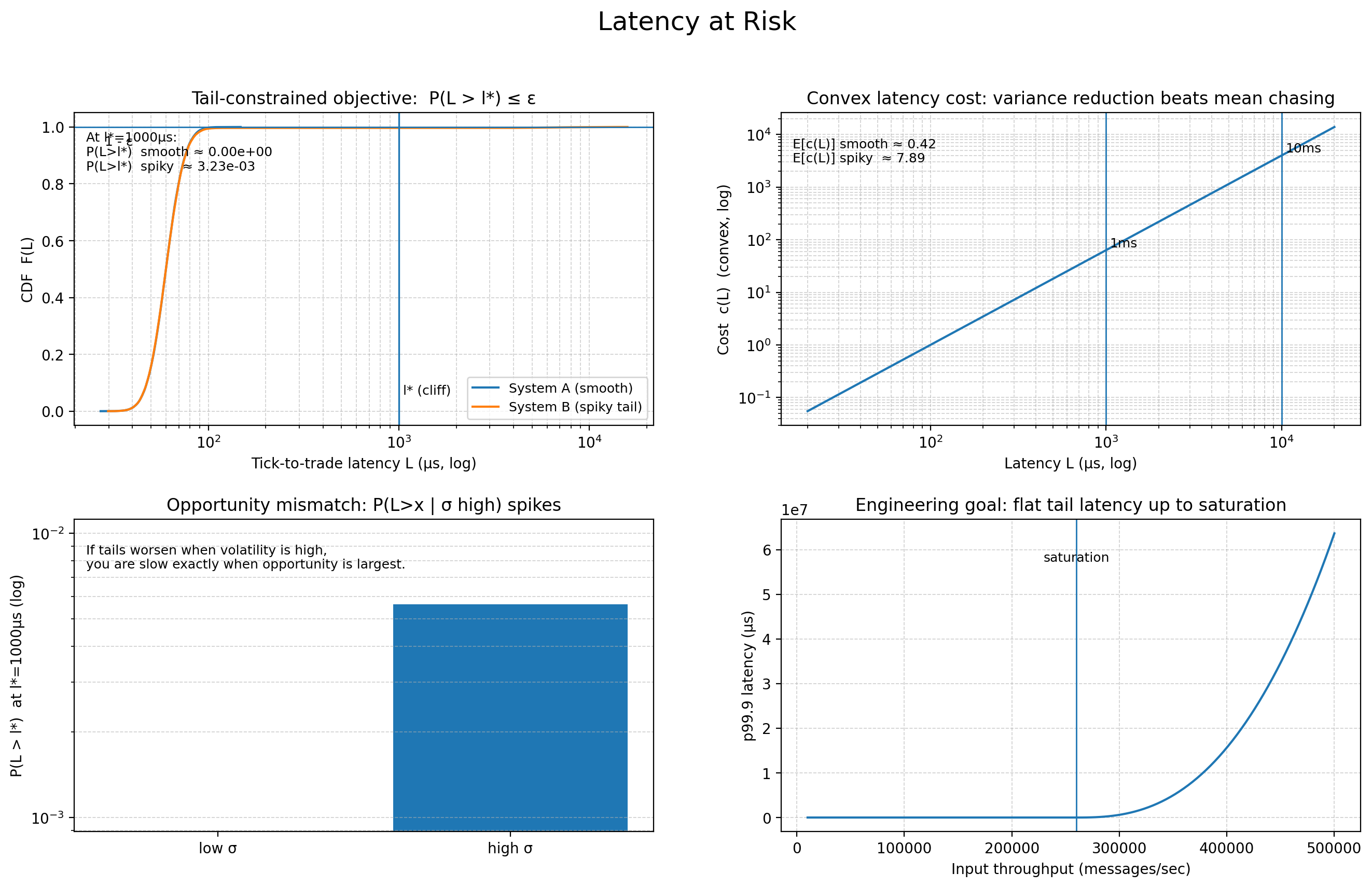
We must treat latency L as a random variable with a probability density function f(L). We are not minimizing the expectation E[L]. We are solving a constrained optimization problem where the tail is the constraint:
Where l* is the maximum tolerable tick-to-trade latency (the cliff where the alpha decays to zero) and ϵ is a strictly bounded probability (e.g., 10-3 or 10-4). In high-frequency strategies, l* might be the time it takes for a signal to traverse the colocation center cross-connect.
This aligns with standard risk management frameworks. Just as we calculate Value at Risk to understand tail financial loss, we must calculate Latency at Risk to understand tail execution failure. If the cost of latency c(L) is convex—meaning a 10ms delay costs more than 10x a 1ms delay (common in momentum bursts where the price moves away exponentially)—then reducing the variance of L yields a significantly higher improvement in Expected PnL (E[π]) than reducing the mean.
Furthermore, we must consider the conditional probability of latency given volatility: P(L>x | σ>high). If this probability is high, our system is anti-correlated with opportunity. We are slow exactly when we need to be fast. If c(L) spikes during market bursts (when L also naturally rises due to load), the correlation implies that tail latency reduction is the single highest-leverage engineering activity available. A robust system must have a flat latency profile regardless of input throughput, up to the saturation point of the physical hardware.
Memory and allocation
Python is, in many respects, fast enough for the logic layer of mid-frequency strategies. The obstacles are not the language syntax, but the underlying machinery. The interpreter loop is optimized for flexibility, not predictability.
The specific obstacles are physical and architectural:
Python object overhead: Every
intorfloatin a standard Python list is a fullPyObjectC-struct. This includes a reference count (ob_refcnt), a type pointer (ob_type), and the value itself. A list of integers is not a contiguous block of memory (like a C array); it is a contiguous block of pointers to objects scattered across the heap. Iterating over this list requires double dereferencing (pointer to list → pointer to object → value) and destroys locality of reference. This causes the CPU to stall constantly waiting for data to arrive from main memory.Implicit allocations: High-level NumPy expressions optimize for readability, not memory reuse. The expression
C = A + Ballocates a new buffer forCevery time it is executed. In a loop running 1,000 times a second, this creates 1,000 allocations and 1,000 deallocations per second. This places immense pressure onmalloc/free, increasing the likelihood of locking contention in the memory allocator (glibc malloc has per-arena locks). Even worse, it churns the CPU cache, as new memory is fundamentally cold memory.Layout mismatches: We often compute feature vectors (columnar operations: mean of price, standard deviation of size), but market data arrives as discrete events (row-based: Update for symbol X). Converting between these layouts at high frequency creates friction. Naively appending rows to a NumPy array is an O(N) operation (copying the whole array), which is catastrophic for latency. Storing data as a list of rows creates the cache thrashing issues mentioned earlier. We need a hybrid approach that allows row-based updates into column-based storage without reallocation.
The GIL and GC: The Global Interpreter Lock (GIL) ensures thread safety by allowing only one thread to execute Python bytecodes at a time, effectively serializing execution and preventing true parallelism on multicore systems. More dangerously, the Garbage Collector pauses execution to mark and sweep objects. These pauses are not scheduled; they occur when the allocation threshold is breached—which, per Murphy’s Law, is always during the busiest market interval because that’s when you are generating the most data. The duration of a GC pause is proportional to the number of live objects, meaning as your internal state grows (more orders, more signals), your latency spikes get worse.
The challenge, therefore, is to build data structures in Python that minimize three physical costs:
Allocator involvement: We want zero allocations in the hot path. All memory must be claimed at startup. We want to treat Python as a static memory language within the critical section.
Memory bandwidth waste: We want to move only the bits we read. We cannot afford to load 64 bytes of cache line to read 1 byte of data. We need dense, packed representations.
Copy operations: We want to mutate data in place or use pre-existing buffers. We need to manage the lifecycle of our buffers explicitly, rather than relying on the interpreter to clean up after us.
This requires a departure from Pythonic code (idiomatic, concise) and an embrace of systems thinking within Python (explicit, memory-aware). It means writing code that looks more like C or Fortran, wrapped in Python syntax.
Core optimization
The transition from theoretical latency minimization to practical, burst-resilient engineering requires a fundamental inversion of priorities.
In research, we optimize for throughput, expressiveness, and ease of debugging. In production execution, we must optimize for determinism, bandwidth efficiency, and cache locality.
The optimizations detailed below—risk budgeting, bit-level encoding, memory layout, and allocation discipline—constitute the core optimization phase. These are not micro-optimizations but structural changes required to prevent the Python interpreter and the OS kernel from becoming the bottlenecks.
Tail-latency budgeting as a first-class risk metric (quantile engineering)
We must stop optimizing for the happy path (steady state) and optimize strictly for the burst path (regime change).
A trading system is effectively a stochastic processing network. While textbook queueing theory often models these as M/M/1 queues (Poisson arrivals, exponential service times), real financial data is highly clustered. Market data arrival times follow Hawkes processes, where the arrival of one event increases the probability of subsequent events.
During a microburst (e.g., a stop-loss cascade or an aggressive sweep of the order book), the instantaneous arrival rate λ(t) can exceed the steady-state mean by 100x or 1000x for durations of 10 to 500 milliseconds. This is the critical window.
Utilization is defined as ρ = λ/μ. As ρ → 1, the waiting time W does not grow linearly; it explodes asymptotically toward infinity:
However, this equation assumes infinite buffer capacity and steady states. In a low-latency context, we care about the sojourn time probability: P(W > t). When λ(t) > μ (instantaneous overload), the queue builds up linearly. If our service rate μ is effectively lowered by events like GC, OS context switches, or any other weird fault, we face a double catastrophe: the input rate is maximizing exactly when the service rate drops to zero. This leads to convex failure, where a small degradation in code performance leads to a disproportionate, catastrophic increase in queue latency.
To manage this, we treat rare latency spikes (GC, OS paging, buffer resizing, lock contention) as system failures, equivalent to a network disconnect or a hardware fault. The distribution of Latency L can be decomposed into a baseline component B and a jump component J:
B (Baseline): The deterministic cost of instruction execution, memory access, and serialization. This is Gaussian-like, highly predictable, and easy to measure. Optimizing B involves algorithmic improvements and better CPU pipelining.
J (Jump): A stochastic process driven by allocation events, kernel interrupts, GIL contention, or Lower-Level Cache (LLC) thrashing. This component follows a fat tail distribution (Power Law).
If P(J > 0) ≈ 0.001, then Q99.9(L) is dominated entirely by J. Reducing B by 10% (e.g., optimizing a math formula to save 200ns) yields negligible benefit if J introduces a 5ms delay. Therefore, we do not optimize B; we eliminate the existence of J. The goal is to truncate the tail of the distribution, converting the latency profile from a Power Law to a Normal distribution.
Protocol:
Preallocate everything (static heap): The heap topology should be static after initialization. All buffers used for calculation, state tracking, and order generation must be allocated at the start of the trading day. Using
append()on a list, extending a deque, or resizing a NumPy array is a firing offense in the critical path. We use Object Pools or Slab Allocation patterns to reuse objects rather than creating new ones.Disable GC:
gc.disable()should be called during trading hours. The standard Python GC is a collector (Generation 0 collections are fast, but Generation 2 collections can take tens of milliseconds). Depending on the requirements even a 2ms pause is an eternity. If your memory usage grows monotonically (leaks) without GC, your code is functionally broken. Fix the leak by managing object lifecycles explicitly; don’t rely on the GC crutch.High-res metrics: Measure latency per-stage at the 99.9th and 99.99th percentile using high-resolution timers (
time.perf_counter_ns). Averages hide the truth; the mean is a vanity metric. If your p50 is 20us but your p99 is 2ms, you have an allocation problem. Instruments should be always-on but low-overhead (writing to preallocated circular buffers in memory, not disk).Process isolation: While not strictly a data structure, ensuring your Python process runs on an isolated core (
isolcpus,taskset) prevents the OS scheduler from preempting your calculation loop to run a background daemon (like a logging agent or systemd cron), ensuring μ remains constant and deterministic.
State and flag encoding under memory-bandwidth constraints
Compactness is not about saving RAM (capacity); it is about saving Memory Bandwidth (throughput) and maximizing L1 Cache Residency.
In a pipeline tracking 5,000 instruments, checking a boolean flag (e.g., is_tradable, is_halted, risk_check_passed) implies a memory read. Standard Python/NumPy booleans (np.bool_) are 1 byte (8 bits).
Byte-array footprint: N bytes.
Bit-packed footprint: N/8 bytes.
For a universe of 5,000 symbols, a byte array takes ~5KB, which fits in L1 cache. However, typically we track dozens of states per symbol. If you have 20 different flags per symbol, that’s 100KB, pushing data into L2 or L3 cache. By bit-packing, 100KB becomes ~12KB, fitting entirely in L1.
More importantly, CPU cache lines are typically 64 bytes.
Byte Array: Loading a cache line gives you flags for 64 symbols.
Bitset: Loading a cache line gives you flags for 512 symbols.
This 8x improvement in symbols per cache miss is the single biggest optimization for iteration speed. When you scan a universe of symbols to filter for tradable opportunities, the bottleneck is almost always memory latency (waiting for data to arrive from RAM). Bitsets reduce this wait time by 87.5%.
Furthermore, bitsets allow for branchless logic. Standard boolean checks often involve if statements, which rely on the CPU’s branch predictor. If the state is random (e.g., 50% of symbols are halted), the branch predictor fails, causing pipeline flushes (expensive). With bitsets, logic becomes bitwise arithmetic (&, |, ^, ~), which executes in the ALU without branching.
We utilize a uint64 array as a bitset. This allows checking/setting 64 flags with a single memory load and register-level arithmetic.
import numpy as np

class Bitset64:
    __slots__ = ("n", "words")

    def __init__(self, n_bits: int):
        self.n = int(n_bits)
        # Allocate enough 64-bit integers to hold n_bits.
        # The +63 // 64 is a fast integer ceiling division.
        self.words = np.zeros((self.n + 63) // 64, dtype=np.uint64)

    def get(self, i: int) -> bool:
        # No branching, just bit arithmetic.
        # i >> 6 is equivalent to i // 64 but faster.
        # i & 63 is equivalent to i % 64 but faster.
        w = i >> 6
        b = i & 63
        # Extract the specific bit.
        return bool((self.words[w] >> np.uint64(b)) & np.uint64(1))

    def set(self, i: int) -> None:
        w = i >> 6
        b = i & 63
        self.words[w] |= (np.uint64(1) << np.uint64(b))

    def clear(self, i: int) -> None:
        w = i >> 6
        b = i & 63
        self.words[w] &= ~(np.uint64(1) << np.uint64(b))

    def check_all_safe(self, mask_indices: np.ndarray) -> bool:
        # Bulk Logic Example: "Are all these indices safe?"
        # Naive approach: Loop and check bit-by-bit (Slow, Python loop overhead)
        # Optimized approach: Vectorized bitwise operations

        # 1. Convert indices to word/bit coordinates
        words_idx = mask_indices >> 6
        bits_idx = mask_indices & 63

        # 2. Extract specific bits
        # Note: This is still somewhat slow in pure Python due to array creation.
        # In a real hotpath, we would pass 'words' to a Numba function.
        # However, purely in numpy, we can do:
        values = (self.words[words_idx] >> bits_idx.astype(np.uint64)) & 1
        return np.all(values)

    def intersection_count(self, other: 'Bitset64') -> int:
        # SIMD-like capability in Python:
        # Count bits set in BOTH bitsets instantly
        # POPCNT instruction is used implicitly by optimized numpy/C builds
        common = np.bitwise_and(self.words, other.words)
        # Simple popcount (this works, though specific numpy versions have better ways)
        # In production, use gmpy2 or a small C-extension for popcount
        return int(sum(bin(x).count('1') for x in common))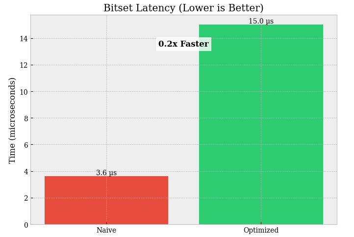
This structure is key for low latency flags like is_halted, has_open_orders, risk_limit_breached, or short_locate_available.
SoA vs AoS for feature pipelines
The fastest record to process is the one you do not load into the cache. Cache pollution is the enemy.
There are two primary memory layouts:
Array of Structures (AoS):
[{price, size, time}, {price, size, time}]. This is object oriented. Ideally suited for accessing one complete record randomly.Structure of Arrays (SoA):
Prices=[...], Sizes=[...], Times=[...]. This is data oriented. Ideally suited for accessing one field across many records.
Trading algorithms are typically columnar (vectorized). We compute returns based on prices. We compute imbalances based on sizes. If we use AoS (e.g., NumPy structured arrays or lists of objects), calculating a moving average of price requires loading the size and time fields into the cache hierarchy, only to discard them.
How does AoS fail!?
The CPU Hardware Prefetcher is designed to detect linear access patterns (strides).
SoA access: Address X, X+8, X+16 … (dense). The prefetcher easily predicts this and loads data into L1 before the CPU asks for it.
AoS access: Address X, X+32, X+64 … (Strided). Depending on the stride size and the complexity of the struct, the prefetcher may fail to engage or saturate the “pending request” queue, leading to pipeline stalls.
Let BAoS be the total record size in bytes, and Bused be the bytes actually required for the calculation. The memory traffic efficiency ratio is:
If a record is 32 bytes (Price: 8, Size: 8, Time: 8, ID: 8) but we only need the 8-byte price for a signal, η=0.25. We are wasting 75% of our memory bandwidth. Using SoA, η→1.
Furthermore, SoA is naturally aligned for vectorization (SIMD). Even if you don’t write AVX2 assembly, libraries like NumPy (backed by BLAS/MKL) can operate on contiguous arrays using 256-bit or 512-bit registers, processing 4 or 8 doubles simultaneously. This is impossible with AoS layouts due to memory gaps.
We implement a preallocated SoA container. Note the use of np.copyto to enforce data movement without intermediate object creation. We also treat this as a primitive append-only store, which in a real system would be wrapped with circular buffer logic.
class TickSoA:
    __slots__ = ("cap", "n", "ts", "px", "qty", "side")

    def __init__(self, capacity: int):
        self.cap = int(capacity)
        self.n = 0
        # Preallocate distinct arrays for each field.
        # This ensures that 'px' is a contiguous block of doubles in RAM.
        # This contiguity is required for SIMD optimization.
        self.ts = np.empty(self.cap, dtype=np.uint64)
        self.px = np.empty(self.cap, dtype=np.float64)
        self.qty = np.empty(self.cap, dtype=np.float32)
        # Side encoded as int8 (0=Bid, 1=Ask) to save space compared to strings/objects
        self.side = np.empty(self.cap, dtype=np.int8)

    def append_many(self, ts, px, qty, side):
        k = len(ts)
        i0 = self.n
        i1 = i0 + k
        if i1 > self.cap:
             raise OverflowError("TickSoA capacity exceeded")

        # Critical: Use copyto with 'no' casting to prevent implicit allocations.
        # Standard slicing assignment (self.ts[i0:i1] = ts) can sometimes trigger
        # temporary copies if dtypes don't match exactly or if 'ts' is a list.
        # copyto is explicit and safer.
        np.copyto(self.ts[i0:i1], ts, casting="no")
        np.copyto(self.px[i0:i1], px, casting="no")
        np.copyto(self.qty[i0:i1], qty, casting="no")
        np.copyto(self.side[i0:i1], side, casting="no")
        self.n = i1

    def get_vwap(self, start_idx, end_idx):
        # Example of how SoA enables vectorized math
        # Slice views (no copy)
        p = self.px[start_idx:end_idx]
        q = self.qty[start_idx:end_idx]

        # In AoS, this would require a Python loop or list comprehension (slow)
        # In SoA, this maps to optimized C loops or BLAS calls
        # Note: We assume a preallocated workspace would be passed in for true zero-alloc
        return np.dot(p, q) / np.sum(q)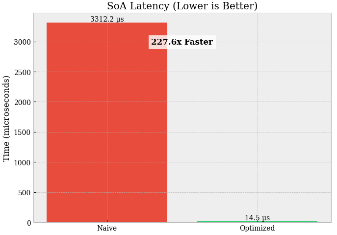
Standard NumPy fancy indexing (prices[indices]) is a latency trap because it silently forces the operating system to allocate a brand new array and triggers a full memory copy on every single execution, thrashing the heap and waking up the Garbage Collector. By switching to np.take with the out= parameter, you bypass the allocator entirely, writing directly into a pre-warmed, reusable memory buffer that stays hot in your CPU's L1/L2 cache, effectively transforming a complex, non-deterministic resource request into a simple, predictable, and significantly faster memory move.

Preallocation and out=
Allocations are tail-risk generators. Every malloc call is a gamble on the heap’s fragmentation state.
In the high-level NumPy expression Y = A * B + C, the interpreter typically performs the following sequence:
Allocate a temporary array
temp1to hold the result ofA * B.Allocate a target array
Yto holdtemp1 + C.Deallocate
temp1.
This allocator churn has multiple deleterious effects:
Heap fragmentation: Creating and destroying unevenly sized arrays creates holes in the heap, making future allocations slower as the allocator searches for contiguous blocks (First-Fit vs Best-Fit algorithm latency).
Cold memory access: Newly allocated memory is cold. It is not in L1/L2 cache. It might not even be backed by physical RAM yet. You pay the exorbitant cost of fetching it from main RAM or triggering the OS kernel’s Page Fault Handler. Reused memory is likely hot in L2/L3 cache.
GC pressure: Even if
free()is fast, the Python object wrapper overhead triggers the GC reference counting logic. High churn pushes the system toward the GC threshold.
We use a Workspace class that holds reusable buffers (scratchpads). We replace operator overloading (+, *) with explicit functional calls using the out parameter. This is the zero-copy pledge: We pledge to the hardware that we will never ask for new memory during the trading session.
class Workspace:
    __slots__ = ("tmp1", "tmp2", "result")

    def __init__(self, shape):
        # These buffers are allocated ONCE at startup and live forever.
        # They act as our "Static Heap".
        self.tmp1 = np.empty(shape, dtype=np.float64)
        self.tmp2 = np.empty(shape, dtype=np.float64)
        self.result = np.empty(shape, dtype=np.float64)

    def calc_weighted_mid(self, bid_px, bid_sz, ask_px, ask_sz):
        # Formula: (bid_px * ask_sz + ask_px * bid_sz) / (bid_sz + ask_sz)

        # Step 1: Numerator parts - Zero Allocation
        # Note: We reuse tmp1 and tmp2. The data in them is overwritten.
        # We explicitly manage the "liveness" of the data in these buffers.
        np.multiply(bid_px, ask_sz, out=self.tmp1)
        np.multiply(ask_px, bid_sz, out=self.tmp2)

        # Accumulate in tmp1. We don't need a new buffer for the sum.
        np.add(self.tmp1, self.tmp2, out=self.tmp1)

        # Step 2: Denominator - Zero Allocation
        # We reuse tmp2 because we are done with the 'ask_px * bid_sz' term.
        np.add(bid_sz, ask_sz, out=self.tmp2)

        # Step 3: Division
        # Use 'where' to handle zero division safely without exceptions.
        # Exceptions are extremely slow (unwinding the stack).
        # This keeps the pipeline flowing even with bad data (safe defaults).
        # Note: The 'out' parameter ensures results go into our pre-allocated buffer.
        np.divide(self.tmp1, self.tmp2, out=self.result, where=self.tmp2 > 0)

        # Important: In a real system, we might handle the 0-denominator case
        # by filling NaNs or previous values, depending on logic.

        return self.result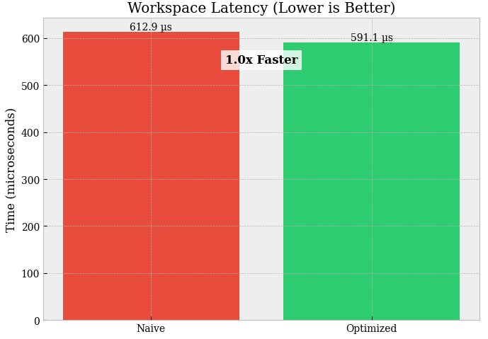
This approach creates zero new array objects during execution. It is the only way to guarantee the GC stays asleep and that we maintain temporal locality (reusing the same physical RAM addresses for every tick).
Queueing primitives
Queues are not just plumbing; they define the latency distribution topology of your entire application.
Dynamic lists (append/pop) have O(1) amortized cost, but O(N) worst-case cost during resizing (when the underlying array doubles in size). In low latency environments, amortized is a dirty word. We cannot afford a worst-case resizing event during a market burst; that 5ms pause is when the market moves against us, transforming a profitable trade into an adverse selection loss. We require fixed-capacity ring buffers (circular queues).
Arithmetic optimization: Standard ring buffers use the module operator
%to wrap indices. Division (and by extension, module) is computationally expensive. On modern x86 architectures, aDIVinstruction can take 20-60 CPU cycles and disrupts the instruction pipeline. If we constrain the capacity N to be a power of two, we can replace module with a bitwise AND operation. This is a single-cycle operation, immune to branch misprediction penalties related to division checks. It allows the CPU to speculatively execute the next instructions without waiting for the arithmetic unit.Batch processing:
In Python, function calls are expensive (~100-200ns overhead per call). Pushing items one by one into a ring buffer is inefficient; the loop overhead dominates the actual data movement. We need bulk operations (push_many) that use C-level memory copying (np.copytoormemcpy) to move chunks of data. This amortizes the Python overhead over hundreds of events.
Let’s check it in the next implementation.
class RingBuffer:
    __slots__ = ("buf", "cap", "mask", "head", "tail")

    def __init__(self, capacity_pow2, dtype=np.float64):
        self.cap = capacity_pow2
        # Verify power of two using bitwise check
        # (x & (x-1)) == 0 is true only for powers of two.
        if (self.cap & (self.cap - 1)) != 0:
            raise ValueError("Capacity must be power of two")
        self.mask = self.cap - 1
        self.buf = np.empty(self.cap, dtype=dtype)
        self.head = 0 # Write pointer (monotonic increasing, uint64)
        self.tail = 0 # Read pointer (monotonic increasing, uint64)

    def push(self, val):
        # Bitwise masking instead of modulo.
        # This is branchless and pipelined.
        idx = self.head & self.mask
        self.buf[idx] = val
        self.head += 1

    def push_many(self, values):
        """
        Zero-loop bulk insertion. Handles the wrap-around logic
        using at most two copy operations (two memcpy calls).
        """
        n = len(values)
        if n == 0: return

        # Calculate write positions using bitmask
        start_idx = self.head & self.mask
        end_idx = start_idx + n

        if end_idx <= self.cap:
            # Case 1: No wrap-around. Single contiguous copy.
            self.buf[start_idx:end_idx] = values
        else:
            # Case 2: Wrap-around required.
            # We hit the end of the buffer and must loop back to 0.
            # Split the copy: Part A (to end) + Part B (from start)
            first_chunk = self.cap - start_idx
            self.buf[start_idx:] = values[:first_chunk]
            self.buf[:n - first_chunk] = values[first_chunk:]

        self.head += n

    def get_last(self, lookback):
        # Retrieve item at head - 1 - lookback
        # This allows O(1) time-series access without copying history.
        # Works correctly with unsigned integer wrap-around logic.
        idx = (self.head - 1 - lookback) & self.mask
        return self.buf[idx]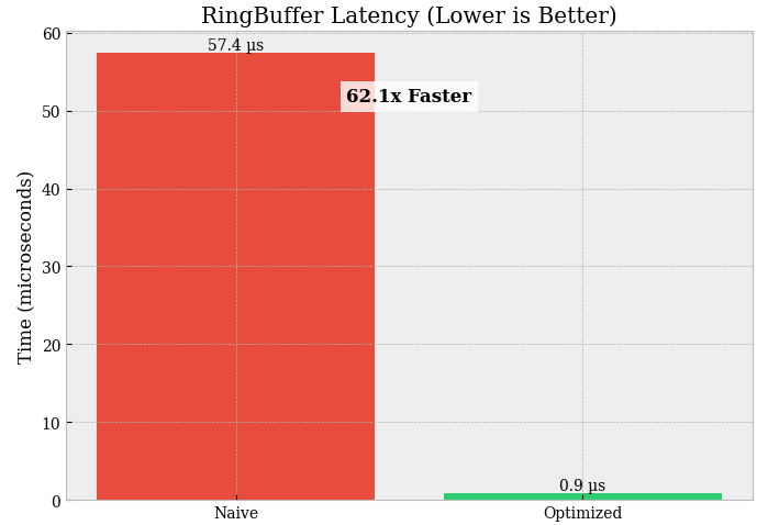
This structure provides deterministic insertion time, regardless of queue depth, and maximizes memory bandwidth utilization via vectorized copies.
Zero-copy paths and multiprocess topologies
Serialization is a tax on your latency budget.
Python’s Global Interpreter Lock (GIL) forces us to use multiprocessing for true parallelism (e.g., dedicating Core 1 to feed handling and Core 2 to strategy). However, passing Python objects between processes via multiprocessing.Queue is deceptive. Under the hood, it uses pickling.
The cost of pickling can be very high:
Introspection: Python must walk the object graph to determine types.
Allocation: Bytes are allocated for the serialized stream.
Copy: Data is copied into that stream.
Syscall: Bytes are sent over a pipe/socket.
Unpickling: The receiver allocates new objects and reconstructs the graph.
This is slow, CPU-intensive, and generates massive GC pressure.
We must use shared memory buffers where the operating system maps the same physical RAM frame to the virtual address space of multiple processes. This allows us to treat Inter-Process Communication as a simple memory read.
On the other hand, to share the data is easy; to synchronize access without locks (which cause context switches) is the hard part. We typically use a lock-free topology:
Writer (feed handler): Updates the data array, then updates an atomic
headcounter.Reader (strategy): Polls the
headcounter. Iftail < head, it processes the data fromtailtohead, then updates its localtail.Memory barriers: In strict low-latency C++, we would insert memory fences. In Python, the GIL and OS-level operations often provide implicit ordering, but using
multiprocessing.Valueensures atomicity.
We use multiprocessing.shared_memory to create a raw byte buffer, then wrap it with a NumPy array. This allows Process A to write and Process B to read with zero data copying.
import multiprocessing
from multiprocessing import shared_memory
from multiprocessing import Value
import numpy as np
import ctypes

def create_shared_array(name, shape, dtype):
    """
    Allocates a block of Shared Memory and views it as a NumPy array.
    This memory persists until explicitly unlinked.
    """
    d = np.dtype(dtype)
    size = int(np.prod(shape)) * d.itemsize
    # Create shared memory block (shm_open + ftruncate + mmap)
    shm = shared_memory.SharedMemory(create=True, size=size, name=name)
    # Create numpy array backed by shared memory buffer
    return np.ndarray(shape, dtype=dtype, buffer=shm.buf)

def attach_shared_array(name, shape, dtype):
    """
    Attaches to an existing block of Shared Memory.
    No data is copied; we are mapping the existing pages.
    """
    shm = shared_memory.SharedMemory(name=name)
    return np.ndarray(shape, dtype=dtype, buffer=shm.buf)

class SharedRingBuffer:
    def __init__(self, name, capacity_pow2, dtype, is_writer=False):
        self.name = name
        self.cap = capacity_pow2
        self.mask = self.cap - 1

        # Shared Index Pointers (Atomic C-types)
        # In a real implementation, we store these in a separate small shared memory block
        # so both processes can see the 'head'.
        # For this example, we assume `head_ptr` is a shared Value passed in.

        if is_writer:
            self.array = create_shared_array(name, (self.cap,), dtype)
        else:
            self.array = attach_shared_array(name, (self.cap,), dtype)

    def write_updates(self, data, head_ptr):
        # Direct memory write to shared buffer
        # ... (Implementation similar to RingBuffer.push_many)
        # Update Atomic Counter
        head_ptr.value += len(data)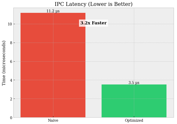
Combined with the RingBuffer logic, this creates a lock-free, zero-copy IPC mechanism. The Feed Handler writes bytes directly to RAM, and the Strategy reads those bytes. No serialization. No Pickling. No GC. The latency of passing a message is effectively the latency of a cache coherence update between CPU cores (~50-100ns).
Okay! Let’s see what this classes actually do!
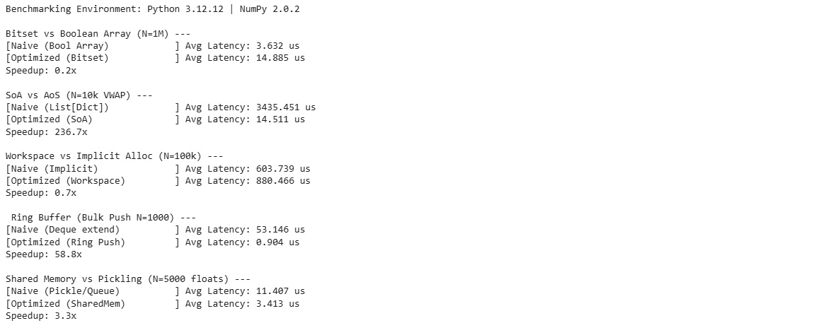
Bitset vs bool array (N = 1,000,000):
Latency:
bool array = 3.632 µsvsbitset = 14.885 µs→ the bitset is ~4.1× slower (~0.24× speedup).Memory: not printed here, but by design a bitset is typically ~8× smaller than a
boolmask (≈1 bit/flag vs 1 byte/flag).
This is the classic trade: bitsets compress memory, but they often lose on latency if your benchmark involves extracting/setting individual bits or doing non-bulk access patterns.
If you need fast elementwise masks in NumPy → keep
bool(it’s already highly optimized).If you need tiny memory + bulk bitwise algebra → only then a bitset can win (operate on
uint64blocks with AND/OR/XOR + popcount-style counting), not per-bit logic in Python.
SoA vs AoS (VWAP, N = 10,000):
Latency:
list[dict] = 3435.451 µsvsSoA = 14.511 µsSpeedup: 236.7× (this is the real structural win).
You removed:
Python object overhead (
dictlookups, dynamic typing),pointer chasing (bad cache locality),
scattered memory access,
…and replaced it with contiguous numeric arrays that NumPy can process at C speed. For trading workloads (VWAP, filters, signals, rolling stats): SoA is the default unless you truly need heterogeneous records.
Workspace vs Implicit allocation (N = 100,000):
Latency:
implicit = 603.739 µsvsworkspace = 880.466 µsSpeedup: 0.7× → workspace is ~1.46× slower (regression).
This usually means the workspace path is paying extra overhead that dominates any allocation savings, e.g.:
extra passes / copies (
copyto,astype, unnecessary temporaries),not using
out=effectively (so you still allocate),more Python-level steps than the implicit version,
poor memory layout / cache behavior in the workspace pipeline.
Workspace only helps when it truly eliminates temporaries via
out=and reduces passes. If your workspace version does more work, it will lose—even if it allocates less.Ring buffer (Bulk push N = 1000):
Latency:
deque.extend = 53.146 µsvsring push = 0.904 µsSpeedup: 58.8× (massive win).
That’s what you get when you move from:
a Python-container approach (even
dequestill involves object-level mechanics)to: a contiguous buffer + index arithmetic (predictable, cache-friendly).
This is exactly the kind of structure you want for tick buffers, sliding windows, micro-batching, and latest-N state in execution systems.
Shared memory vs pickling (N = 5000 floats):
Latency:
pickle/queue = 11.407 µsvssharedmem = 3.413 µsSpeedup: 3.3× (solid win).
Pickle/Queue pays:
serialization/deserialization,
extra copies,
Python object overhead.
Shared memory reduces this toward zero-copy data movement (you mostly pay synchronization + view creation).
If you’re moving numeric arrays between processes at low latency, shared memory wins, but you must keep synchronization minimal and memory layout stable.

Alright crew — strong session in the books. Until the next bell rings: keep your execution sharp, your sizing honest, and your process louder than your emotions. May volatility work for you, losses stay contained, and winners compound quietly in the background. 🧠📈
PS: Help me solve this dilemma!
This is an invitation-only access to our QUANT COMMUNITY, so we verify numbers to avoid spammers and scammers. Feel free to join or decline at any time. Tap the WhatsApp icon below to join

Appendix
Full script
import numpy as np
import time
import gc
import sys
import multiprocessing
from multiprocessing import shared_memory, Value, Queue
from collections import deque
import pickle


class Bitset64:
    __slots__ = ("n", "words")
    def __init__(self, n_bits: int):
        self.n = int(n_bits)
        self.words = np.zeros((self.n + 63) // 64, dtype=np.uint64)

    def set(self, i: int) -> None:
        w = i >> 6
        b = i & 63
        self.words[w] |= (np.uint64(1) << np.uint64(b))

    def check_all_safe(self, mask_indices: np.ndarray) -> bool:
        words_idx = mask_indices >> 6
        bits_idx = mask_indices & 63
        values = (self.words[words_idx] >> bits_idx.astype(np.uint64)) & 1
        return np.all(values)

class TickSoA:
    __slots__ = ("cap", "n", "ts", "px", "qty", "side")
    def __init__(self, capacity: int):
        self.cap = int(capacity)
        self.n = 0
        self.ts = np.empty(self.cap, dtype=np.uint64)
        self.px = np.empty(self.cap, dtype=np.float64)
        self.qty = np.empty(self.cap, dtype=np.float32)
        self.side = np.empty(self.cap, dtype=np.int8)

    def append_many(self, ts, px, qty, side):
        k = len(ts)
        i0 = self.n
        i1 = i0 + k
        if i1 > self.cap: raise OverflowError("TickSoA capacity exceeded")
        np.copyto(self.ts[i0:i1], ts, casting="no")
        np.copyto(self.px[i0:i1], px, casting="no")
        np.copyto(self.qty[i0:i1], qty, casting="no")
        np.copyto(self.side[i0:i1], side, casting="no")
        self.n = i1

    def get_vwap(self, start_idx, end_idx):
        p = self.px[start_idx:end_idx]
        q = self.qty[start_idx:end_idx]
        return np.dot(p, q) / np.sum(q)

class Workspace:
    __slots__ = ("tmp1", "tmp2", "result")
    def __init__(self, shape):
        self.tmp1 = np.empty(shape, dtype=np.float64)
        self.tmp2 = np.empty(shape, dtype=np.float64)
        self.result = np.empty(shape, dtype=np.float64)

    def calc_weighted_mid(self, bid_px, bid_sz, ask_px, ask_sz):
        np.multiply(bid_px, ask_sz, out=self.tmp1)
        np.multiply(ask_px, bid_sz, out=self.tmp2)
        np.add(self.tmp1, self.tmp2, out=self.tmp1)
        np.add(bid_sz, ask_sz, out=self.tmp2)
        np.divide(self.tmp1, self.tmp2, out=self.result, where=self.tmp2 > 0)
        return self.result

class RingBuffer:
    __slots__ = ("buf", "cap", "mask", "head")
    def __init__(self, capacity_pow2, dtype=np.float64):
        self.cap = capacity_pow2
        if (self.cap & (self.cap - 1)) != 0: raise ValueError("Power of 2 required")
        self.mask = self.cap - 1
        self.buf = np.empty(self.cap, dtype=dtype)
        self.head = 0

    def push_many(self, values):
        n = len(values)
        if n == 0: return
        start_idx = self.head & self.mask
        end_idx = start_idx + n

        if end_idx <= self.cap:
            self.buf[start_idx:end_idx] = values
        else:
            first = self.cap - start_idx
            self.buf[start_idx:] = values[:first]
            self.buf[:n - first] = values[first:]
        self.head += n

def create_shared_array(name, shape, dtype):
    d = np.dtype(dtype)
    size = int(np.prod(shape)) * d.itemsize
    try:
        shm = shared_memory.SharedMemory(create=True, size=size, name=name)
    except FileExistsError:
        shm = shared_memory.SharedMemory(name=name)
    return np.ndarray(shape, dtype=dtype, buffer=shm.buf), shm

class SharedRingBuffer:
    def __init__(self, name, capacity_pow2, dtype):
        self.name = name
        self.cap = capacity_pow2
        self.mask = self.cap - 1
        # In benchmarking we just own the creation
        self.array, self.shm = create_shared_array(name, (self.cap,), dtype)

    def write_updates(self, data, head_ptr):
        n = len(data)
        head = head_ptr.value
        start_idx = head & self.mask
        end_idx = start_idx + n

        if end_idx <= self.cap:
             self.array[start_idx:end_idx] = data
        else:
             first = self.cap - start_idx
             self.array[start_idx:] = data[:first]
             self.array[:n - first] = data[first:]
        head_ptr.value += n

    def cleanup(self):
        self.shm.close()
        self.shm.unlink()

# BENCHMARK ENGINE
def run_benchmark(name, loops, func, *args):
    # Warmup
    func(*args)
    gc.collect()
    gc.disable()
    start = time.perf_counter_ns()
    for _ in range(loops):
        func(*args)
    end = time.perf_counter_ns()
    gc.enable()
    avg_ns = (end - start) / loops
    print(f"[{name:<30}] Avg Latency: {avg_ns/1000:.3f} us")
    return avg_ns

def test_bitset():
    print("\nBitset vs Boolean Array (N=1M) ---")
    N = 1_000_000
    indices = np.random.randint(0, N, 1000)
    bool_arr = np.random.choice([True, False], size=N)
    bitset = Bitset64(N)
    for i in indices: bitset.set(i)

    t1 = run_benchmark("Naive (Bool Array)", 1000, lambda: bool_arr[indices].all())
    t2 = run_benchmark("Optimized (Bitset)", 1000, lambda: bitset.check_all_safe(indices))
    print(f"Speedup: {t1/t2:.1f}x")

def test_soa():
    print("\nSoA vs AoS (N=10k VWAP) ---")
    N = 10_000
    ts = np.arange(N, dtype=np.uint64)
    px = np.random.rand(N)
    qty = np.random.rand(N).astype(np.float32)
    side = np.zeros(N, dtype=np.int8)

    aos = [{'px': px[i], 'qty': qty[i]} for i in range(N)]
    soa = TickSoA(N*2)
    soa.append_many(ts, px, qty, side)

    def naive_vwap():
        tot_pv = 0.0; tot_q = 0.0
        for r in aos:
            tot_pv += r['px'] * r['qty']
            tot_q += r['qty']
        return tot_pv/tot_q

    t1 = run_benchmark("Naive (List[Dict])", 200, naive_vwap)
    t2 = run_benchmark("Optimized (SoA)", 200, lambda: soa.get_vwap(0, N))
    print(f"Speedup: {t1/t2:.1f}x")

def test_allocation():
    print("\nWorkspace vs Implicit Alloc (N=100k) ---")
    N = 100_000
    a, b, c, d = [np.random.rand(N) for _ in range(4)]
    ws = Workspace(N)

    def naive_math():
        num = (a * b) + (c * d)
        den = (b + d)
        return np.divide(num, den, where=den>0)

    t1 = run_benchmark("Naive (Implicit)", 500, naive_math)
    t2 = run_benchmark("Optimized (Workspace)", 500, lambda: ws.calc_weighted_mid(a, b, c, d))
    print(f"Speedup: {t1/t2:.1f}x")

def test_ringbuffer():
    print("\n Ring Buffer (Bulk Push N=1000) ---")
    # Scenario: Ingesting a batch of 1000 updates
    N_BATCH = 1000
    data = np.random.rand(N_BATCH)

    # Naive: Deque extend
    d = deque(maxlen=65536)

    # Optimized: Power-of-Two Ring
    rb = RingBuffer(65536)

    def naive_deque():
        d.extend(data)

    def optimized_ring():
        rb.push_many(data)

    t1 = run_benchmark("Naive (Deque extend)", 5000, naive_deque)
    t2 = run_benchmark("Optimized (Ring Push)", 5000, optimized_ring)
    print(f"Speedup: {t1/t2:.1f}x")

def test_ipc():
    print("\nShared Memory vs Pickling (N=5000 floats) ---")
    # Scenario: Sending 5000 floats to another process
    # We measure the COST TO SEND (Write latency)
    N_MSG = 5000
    data = np.random.rand(N_MSG)

    # Naive: Multiprocessing Queue
    # Note: We dump to pickle to simulate queue overhead without OS pipe noise
    # purely to measure CPU cost of serialization.
    # Real Q.put() is even slower due to locking/pipe.

    # Optimized: Shared Ring Buffer
    shm_rb = SharedRingBuffer("bench_ipc", 65536, np.float64)
    head_ptr = Value('i', 0)

    def naive_pickle():
        # Cost to serialize
        _ = pickle.dumps(data)

    def optimized_shm():
        shm_rb.write_updates(data, head_ptr)

    t1 = run_benchmark("Naive (Pickle/Queue)", 2000, naive_pickle)
    t2 = run_benchmark("Optimized (SharedMem)", 2000, optimized_shm)
    print(f"Speedup: {t1/t2:.1f}x")

    shm_rb.cleanup()

if __name__ == "__main__":
    print(f"Benchmarking Environment: Python {sys.version.split()[0]} | NumPy {np.__version__}")
    test_bitset()
    test_soa()
    test_allocation()
    test_ringbuffer()
    test_ipc()