[WITH CODE] Switch-off: Robust changepoint protocol
A robust changepoint-based switch-off protocol for algorithmic trading
Table of contents:
Introduction.
The drift in algorithm performance.
Taxonomy of performance drift.
Model risks and limitations.
Robust estimation and the biweight loss.
M-estimators and the geometry of influence.
Tukey’s Biweight (bisquare) loss.
Iteratively Reweighted Least Squares (IRLS).
Regime segmentation via penalized dynamic programming.
The PELT Algorithm (Pruned Exact Linear Time).
The pruning inequality.
Phase 1: Cost Matrix precomputation.
Phase 2: The PELT solver.
Reconstruction and visualizing the drift.
Logic A: Relative decay (alpha erosion).
Logic B: Absolute failure (negative expectancy).
Introduction
Every live strategy is a slowly degrading asset. Not because the model was bad, but because the market keeps changing.
When we deploy an algorithm, we behave as if the distribution that generated its backtest will hang around just long enough for us to harvest the edge. We roll windows, we recalibrate, we monitor drawdowns and Sharpe ratios—all under an implicit truce: whatever drives our PnL won’t change too fast. In practice, that truce is routinely violated.
Edges are conditional stories about the world. Microstructure, liquidity, crowding, policy, fees, latency, and even hardware shape the conditional law that turns a set of signals into returns. Those conditions drift. Sometimes slowly, as competitors discover the same inefficiency and squeeze the juice out of it. Sometimes brutally, as a change in market structure or regulation flips the sign of the trade overnight. From the PnL point of view, both scenarios look like one thing: a strategy that once worked… now doesn’t.
The core operational problem is simple to state and hard to solve:
When does a drawdown stop being noise and become a structural break?
Look at it from the supervisor’s perspective. You observe a noisy sequence of PnL: good days, bad days, occasional 5–10σ events courtesy of fat tails and slippage. Somewhere inside that, the expected value of the strategy can jump from strongly positive to mildly positive, from mildly positive to mediocrity, or from mediocrity to outright negative. Your job is to distinguish those regime changes from random turbulence—fast enough to avoid ruin, slow enough to avoid killing healthy engines.
Standard risk tools are not built for this. Sharpe ratio, volatility targeting, VaR and its cousins are all about dispersion. They tell you how wild the ride is, not whether the underlying game has changed. In fat-tailed, heteroscedastic PnL, a violent loss is weak evidence of anything. A single execution error or fat-finger trade can destroy your mean while telling you nothing about the underlying alpha. Naive responses—Z-score kill switches, rolling-window Sharpe cutoffs, 3σ and you’re out—confuse outliers with structural decay.
At the same time, humans are terrible at making this call in real time. Six months of research sunk into a model, a couple of decent years in production, a rough patch that might be noise or might be decay. The quant knows the theory, the PM sees the drawdown, the committee wants just a bit more evidence. So the strategy stays on. One more week. One more month. One more quarter. By the time everyone agrees it’s dead, the damage is already done.
This article is about replacing that improvisation with a protocol. The implementation was inspired by this paper
Although several modifications were made for our purpose (switch-off tool). Therefore, it is not exactly the same nor does it serve to detect the same thing.
The drift in algorithm performance
A pervasive working assumption in quantitative trading is not full stationarity, but some degree of structural persistence. When we calibrate a model, we estimate parameters θ on a historical sample under the practical assumption that the conditional law driving decisions will not change too fast:
at least in the parts of the state space that matter for our strategy. Even when we use rolling windows, online learning, or adaptive rebalancing, we are implicitly assuming that concept drift is slower than our learning and turnover cycle—that we can track the moving target before we hit a ruin boundary.
In the markets this is, at best, an approximation and often a dangerous one. The return-generating mechanism is subject to regime shifts, structural breaks, policy interventions, technological change, and competition for the same signals. Alpha is not literally defined as a disequilibrium, but operationally it behaves like one:
It is a predictable deviation from what competing capital currently prices in. In a frictionless, unconstrained market, any such predictable excess return is self-destructive: as capital scales into the trade, the pattern is arbitraged away, its Sharpe collapses, and its behaviour migrates towards noise.
This means that alpha decay is not a bug in the research process but the default equilibrium outcome. A deployed strategy is engaged in a race between three clocks:
The decay time of the inefficiency as others discover and crowd it.
The adaptation time of our models and infrastructure.
The risk horizon over which drawdowns become existential.
Stationarity, in this light, is not a realistic global assumption but a local, temporary truce between these clocks. Robust design does not assume that P(X, y) is stationary; it assumes that edges have a finite half-life, and builds everything—the research loop, deployment, and switch-off logic—around surviving long after the original pattern has started to die.
Empirical observation across multiple asset classes—from market making to low-frequency statistical arbitrage—suggests that strategies do not fade linearly. Instead, they exhibit distinct, abrupt regimes. A strategy typically oscillates between:
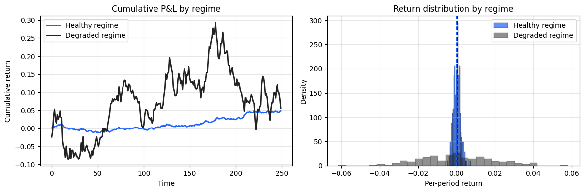
Healthy regime: Positive expectancy (E[r] > 0), stable variance (σ2 ≈ constant), and high information ratio.
Degraded regime: Zero or negative expectancy, often accompanied by volatility clustering where variance spikes due to liquidity constraints, crowding, or breakdown in the correlation structure.
The trader’s dilemma arises when the realized PnL sequence R = {r1, r2, …, rt} deviates from the expected value E[R]. The operator is essentially solving a high-stakes signal classification problem in real-time, often under immense psychological pressure and incomplete information:
Hypothesis H0 (null hypothesis - noise): The deviation is merely sampling variance. The strategy’s edge is intact (E[r] > 0). The drawdown is a statistical artifact of the variance, not a bias in the mean. Action: Do nothing.
Hypothesis H1 (alternative hypothesis - broken): The deviation is structural. The strategy’s edge has evaporated (E[r] ≤ 0). The drawdown is a function of a new, adverse mean. Action: Halt trading.
Because financial time series exhibit high kurtosis (fat tails) and heteroscedasticity (changing variance), a large negative return rt provides surprisingly weak evidence for H1 in isolation. A standard 3σ event—which happens once every 740 years in a Gaussian world—might occur every month in a live trading strategy. Consequently, standard variance-based risk metrics (like Value at Risk, Sharpe Ratio, or volatility targeting) usually fail in this specific context because they measure the magnitude of the dispersion, not the shift in the underlying data generating process.
Taxonomy of performance drift
To correctly diagnose the failure of a strategy, we must move beyond generic labels like drawdown or bad luck and categorize the statistical nature of the failure. We define two primary categories of drift that necessitate a switch-off protocol.
In the previous article, we discussed the different types of drift from a time series perspective, in our case, PnL. Take a look:
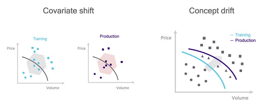
Covariate drift → environmental shift.
Covariate drift occurs when the distribution of the inputs P(X) changes while the conditional probability of the target P(y|X) remains constant.
The market environment shifts, starving the model of its necessary preconditions. Consider a Mean Reversion strategy trained on high-volatility regimes (Xtrain ∼ N(0, σhigh). If the market enters a prolonged period of low volatility (central bank pinning, summer doldrums), the distribution of spread opportunities P(X) collapses.
The strategy’s logic remains mathematically sound—if a spread did open, it would likely close—but the opportunities simply do not arise. The PnL flatlines. However, because the strategy effectively pays rent (server costs, data fees, minimum commissions, and slippage on desperate fills), the net PnL begins to bleed slowly.
This is often termed regime mismatch. While the alpha is not strictly broken, the capital is inefficiently deployed. The correct response may be to hibernate the strategy rather than kill it, but from a PnL perspective, it must be switched off to preserve Sharpe.
Concept drift → alpha decay
Concept drift occurs when the relationship between the signal and the target changes, i.e., P(y|X) shifts. This is the most dangerous form of drift.
The market structure evolves, or the signal becomes crowded.
Example 1 (crowding): A proprietary signal based on order book imbalance worked when you were the only user. Now, five hedge funds are using the same signal. The predictive power X is still visible, but by the time you execute, the price impact of competitors has erased the profit margin. P(y>0|X) drops to near zero.
Example 2 (microstructure): A strategy relies on a latency arbitrage between two exchanges. The exchange updates its matching engine, reducing the latency delta. The physical reality of the arb disappears.
The strategy continues to take trades that look historically valid, but the expected return of those trades shifts from positive to negative. The PnL exhibits a persistent negative trend (drift) that is statistically distinguishable from zero.
This is a structural break. The alpha is dead. No amount of parameter retuning will fix a broken thesis. This requires immediate, permanent cessation of trading.
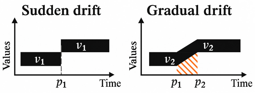
The speed of the drift determines the difficulty of detection.
Gradual drift (the boiled frog): Typical of alpha decay due to competition. The Sharpe ratio erodes from 2.0 to 1.5 to 1.0 over a period of months. This is the hardest to detect because each incremental drop is masked by the daily noise. The operator rationalizes it as a slightly tough month, failing to integrate the long-term trend.
Sudden drift (the cliff edge): Typical of structural breaks, such as a regulatory ban on a specific order type, a change in the maker-taker fee model, or a shift in the tick size. The mean PnL jumps instantaneously from μpositive to μnegative. While the magnitude is larger, the suddenness makes it easier to detect with changepoint algorithms, provided they are robust to outliers.
Our Robust Changepoint Detection model (RCD) is specifically designed to distinguish these structural drifts from mere volatility expansion.
In the absence of a rigorous framework, the decision to stop is psychological rather than statistical. This leads to the sunk cost behavior pattern, well-documented in behavioral finance but particularly acute in quantitative R&D. A quant team may spend 6 months developing a model. When it degrades, the emotional cost of admitting the 6 months of work is now obsolete is incredibly high.
The quant observes a degradation in performance but delays the switch-off decision, waiting for one more data point to confirm the trend. This one more data point is a statistical fallacy; in a noisy time series (Signal-to-Noise << 1), a single point contributes almost zero information gain regarding the regime hypothesis.
This delay is the pivotal source of excess loss in quantitative funds. The conflict is between the human desire for continuity (and the ego associated with the model’s creation) and the statistical reality of the data. We resolve this conflict by removing the human operator from the decision loop entirely. The pivotal event is the automated execution of the switch-off signal, driven purely by the posterior probability of a regime change. The supervisor code becomes the final arbiter of the strategy’s life, acting as a meta-strategy that trades the portfolio of sub-strategies.
Model risks and limitations
While the RCD protocol significantly reduces the risk of ruin compared to naive stop-loss heuristics, it is not a panacea. It introduces a secondary layer of model risk. We are effectively trading one set of assumptions (market stationarity) for another (regime stationarity and independence). Understanding the boundaries of this model is as critical as understanding the strategy it supervises.
The standard formulation of the PELT algorithm, as implemented in this protocol, assumes that the residuals within a regime are Independent and Identically Distributed (i.i.d): ϵt ∼ N(0, σ).
Algorithmic trading PnL is rarely i.i.d.
Mean Reversion Strategies often exhibit negative autocorrelation.
Trend Following Strategies often exhibit positive autocorrelation (streaks/momentum).
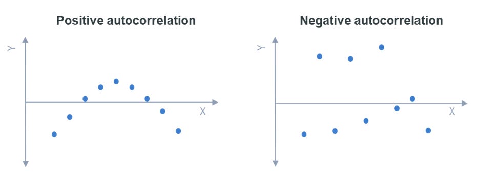
Positive autocorrelation reduces the effective sample size. If a strategy has a lucky streak (autocorrelated wins), the PELT algorithm may interpret this cluster of wins as a distinct high alpha regime. When the streak inevitably reverts to the mean, the algorithm detects a regime shift downwards. This leads to over-segmentation. We detect shifts that are merely artifacts of the serial dependence, leading to potential Type I errors (premature switch-off).
For highly autocorrelated strategies, the PnL series should ideally be pre-whitened or the penalty parameter must be inflated to account for the reduced degrees of freedom.
Besides, the system’s decision boundary is heavily dependent on two hyperparameters: the penalty and the robustness scale K. We typically calibrate K based on a long-term estimate of volatility. However, volatility itself is regime-dependent.
If the market transitions from a low-vol to a high-vol regime without a change in expectancy (Signal-to-Noise drops, but Mean is stable), a static K may interpret the new normal variance as a series of outliers. The biweight loss function will “clip” these valid data points, causing the estimator to become unresponsive or erratic.
The current implementation assumes a relatively homoscedastic noise structure within regimes or relies on the Biweight to simply ignore heteroscedasticity. It does not explicitly model changing volatility regimes as distinct from mean regimes.
The protocol provided is explicitly a switch-off logic. It acts as a circuit breaker. It does not provides a signal for re-entry.
If the supervisor switches off a strategy due to a detected negative drift (Type II Drift), and the strategy subsequently recovers in a simulation-trading environment, the algorithm offers no criteria for reactivation.
There is a significant risk of missing the recovery. Strategies often decay due to temporary crowding and recover when competitors exit (the “ecological cycle” of alpha). By automating the exit but leaving the re-entry to human discretion, we introduce a new behavioral bias: the fear of re-engaging with a failed strategy. This asymmetry can lead to under-allocation during the strategy’s renaissance.
Robust estimation and the biweight loss
In the domain of financial time series, the Ordinary Least Squares estimator is dangerously fragile. While it is the Maximum Likelihood Estimator for Gaussian distributions, its performance degrades catastrophically in the presence of heavy-tailed noise.
To quantify this fragility, we utilize the statistical concept of the breakdown point. The breakdown point of an estimator is the smallest fraction of observations that need to be replaced by arbitrary values to cause the estimator to take on an arbitrarily large value (i.e., to become useless).
The breakdown point of the arithmetic mean is 1/n (asymptotically 0). This implies that a single data point, if sufficiently large, can pull the sample mean to infinity.
The breakdown point of the median is 0.5 (50%). Half the data must be corrupted before the median becomes unreliable.
Consider a strategy with a Sharpe ratio of 2.0. In a typical window of 100 trades, it generates returns clustered tightly around a mean of +0.05R. Our scenario would be something like: A single execution error results in a -50R loss.
Result (mean): The sample mean for the window instantly drops to negative territory. A variance-based switch-off logic (like a Z-score) immediately triggers.
Result (robust): A robust estimator identifies the -50R event as distinct from the data generating process of the alpha. It isolates the outlier, discards it, and correctly identifies that the remaining 99 trades still exhibit a +0.05R expectancy.
The switch-off logic must fundamentally distinguish between execution failure (an outlier) and alpha decay (a shift in the central tendency). The sample mean conflates these two errors.
M-estimators and the geometry of influence
We employ M-estimators, a broad class of estimators obtained as the minima of sums of functions of the data. We minimize an objective function of the form:
where ρ is a symmetric, positive-definite loss function. The choice of ρ dictates the geometry of the risk surface and how the model reacts to deviations.
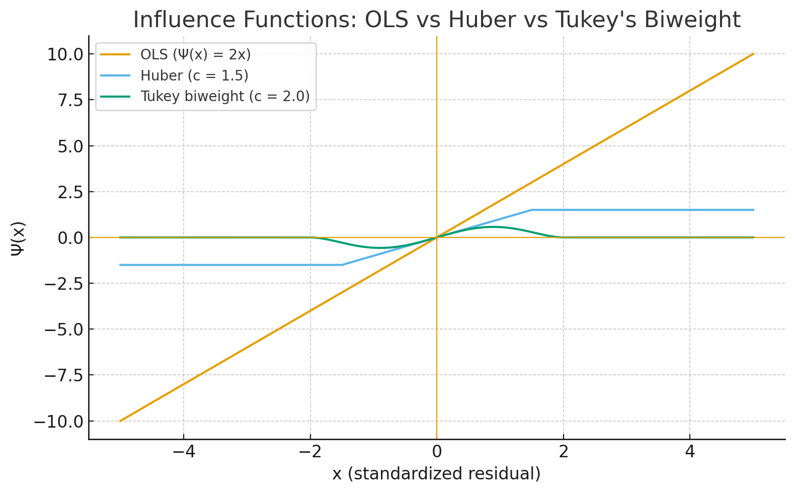
The sensitivity of the estimator to an outlier at value x is described by its influence function, which is proportional to the derivative of the loss function, Ψ(x) = ρ’(x).
Ordinary Least Squares: ρ(x) = x2.
Ψ(x) = 2x.
The influence of an error grows linearly with its magnitude. A 10σ event has 10 times the pull of a 1σ event. This is unacceptable for fat-tailed markets.
Huber Loss: ρ(x) is quadratic for small x and linear for large x.
Ψ(x) = c · sgn(x) for |x|>c.
The influence of an outlier is capped (constant). While better than OLS, it still allows extreme outliers to exert some influence on the location estimate. In a regime switch-off context, even a constant pull from a massive outlier can bias the decision.
Tukey’s Biweight:
Ψ(x) → 0 as |x| → ∞.
This is a redescending M-estimator. Once a data point is identified as being “too far” (beyond a threshold K), its influence completely vanishes. The estimator effectively performs a soft trim, ignoring the data point entirely. This is the property required for a reliable switch-off mechanism.
Tukey’s Biweight (bisquare) loss
To achieve maximum resistance to toxic flow and outliers, we utilize Tukey’s Biweight loss function.
The Biweight loss function is defined as:
The corresponding influence function Ψ(x) is:
Crucially, Ψ(x) = 0 for |x| > K.
The parameter K is not arbitrary; it represents the scale of robustness. It defines the boundary between noise (which affects the mean) and structural breaks/outliers (which should be ignored).
Typically, K is calibrated to c x Scale, where Scale is often the Median Absolute Deviation.
A common default is c=4.685 for asymptotic efficiency at the Normal distribution, but in trading, we often tighten this to c ≈ 2.5 to be more aggressive in rejecting outliers.
Iteratively Reweighted Least Squares (IRLS)
The Biweight loss function is non-convex. This means there is no closed-form solution (like the normal equations for OLS). We must solve for the location parameter θ iteratively.
We utilize the IRLS method. The logic proceeds as follows:
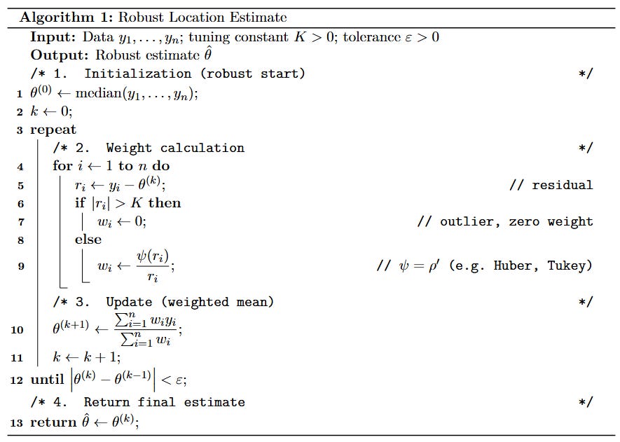
For computational simplicity and speed in our Python implementation (specifically to avoid complex iterative solvers in the inner loop of the dynamic programming step), we approximate the Biweight behavior using a truncated quadratic loss. This effectively clips the influence of any data point beyond distance K from the center.
This function preserves the core property we need: it is quadratic near zero (efficient for Gaussian noise in normal regimes) but constant for large |r| (robust to outliers).
We implement a simplified IRLS solver. Note the specific handling of the mask which serves as a binary weight (0 or 1) rather than the smooth polynomial weight of the full Biweight. This hard rejection is computationally faster and often preferred in high-noise signal processing.
def robust_mean_biweight(y, K, max_iter=50, tol=1e-6):
“”“
Approximate minimiser of sum_i min((y_i - theta)^2, K^2)
using a simple iterative truncated mean.
Parameters
----------
y : array_like
PnL values in one segment.
K : float
Biweight threshold. Residuals with |y_i - theta| >= K are saturated.
max_iter : int
Maximum iterations.
tol : float
Convergence tolerance.
Returns
-------
theta_hat : float
Robust mean estimate for the segment.
“”“
y = np.asarray(y, dtype=float)
if y.size == 0:
return np.nan
# Start from median for robustness
theta = np.median(y)
for _ in range(max_iter):
r = y - theta
mask = np.abs(r) < K # inliers
if not np.any(mask):
# everything is considered an outlier at this theta
return theta
theta_new = y[mask].mean()
if abs(theta_new - theta) < tol:
return theta_new
theta = theta_new
return theta
def biweight_segment_cost(y, K):
“”“
Biweight segment cost and corresponding robust mean.
Cost: sum_i min((y_i - theta)^2, K^2), theta via robust_mean_biweight.
“”“
y = np.asarray(y, dtype=float)
theta = robust_mean_biweight(y, K)
r = y - theta
loss = np.where(np.abs(r) < K, r**2, K**2)
return float(loss.sum()), thetaIt is critical to note that the Biweight loss function is non-convex. Unlike OLS (a simple bowl shape), the Biweight loss surface has multiple local minima.
If we initialize the IRLS algorithm with an arbitrary value (e.g., zero, or the previous window’s mean), the solver might get stuck in a local minimum that corresponds to a cluster of outliers rather than the main data distribution.
This is why the code explicitly initializes theta = np.median(y). The median is guaranteed to be close enough to the global minimum to place the solver within the basin of attraction of the true robust mean.
Regime segmentation via penalized dynamic programming
We have shifted our perspective from viewing PnL as a continuous random walk to viewing it as a discrete sequence of distinct structural regimes. This discretization is a fundamental assertion about the nature of market dynamics.
Let y1:n be the sequence of realized PnL returns. We assume the existence of a set of m changepoints τ1, …, τm that partition the historical data into m+1 discrete segments. Within the j-th segment, defined by the interval (τj-1, τj], the data is modeled as independent and identically distributed (i.i.d.) with a specific location parameter θj and scale parameter σj.
Our operational goal is to identify the optimal set of changepoints. This is fundamentally an optimization problem where we must balance two competing forces: Fidelity (how well the model fits the data) and parsimony (the simplicity of the model).
Let C(ys:e) denote the aggregate robust cost—calculated as the summation of individual biweight loss contributions—for a candidate market regime. This segment is rigorously defined by the temporal interval initiating at index s (representing the hypothesized genesis of a new statistical environment) and extending through to index e. In this context, s serves as the critical boundary condition: it is the candidate time-step where the algorithm postulates that the prior market dynamics have structurally decoupled from the future. At index s, the joint distribution P(Xs-1, ys-1) is assumed to diverge from P(Xs, ys), necessitating the estimation of a new location parameter θ for the subsequent window.
We seek to minimize the following penalized objective function:
Here, β is the penalty term, functioning as a regularizer similar to the role of λ in Ridge Regression or the penalty in the Akaike Information Criterion.
The Fit (C): This term pushes the model to add more changepoints. In the limit, if we assign a distinct regime to every single data point, the cost C drops to zero (perfect fit).
The Regularizer (β): This term penalizes complexity. It imposes a cost for declaring a regime change.
The optimization landscape is defined by the interaction of these terms:
If β → 0, the cost function is dominated by the fit. The optimal solution converges to a changepoint at every time step t, modeling noise as structure (overfitting).
If β → ∞, the penalty dominates. The optimal solution collapses to zero changepoints, modeling the entire history as a single stationary regime (underfitting).
The PELT Algorithm (Pruned Exact Linear Time)
Finding the global minimum of the objective function via brute force is computationally intractable. For a time series of length n, there are 2n-1 possible segmentations.
For n=100 trades, this is 299 combinations—a number exceeding the estimated number of atoms in the universe.
Consequently, heuristic methods (like sliding windows) are often used, but they fail to guarantee global optimality and are sensitive to window size.
However, the problem exhibits optimal Substructure: the optimal segmentation of the entire history y1:t contains within it the optimal segmentation of a sub-problem ending at some previous time s. This allows us to utilize Dynamic Programming (DP).
Here is where the Bellman’s Principle of Optimality comes into action. We define F(t) as the minimum cost of segmenting the data from the start up to time t. The recurrence relation (Bellman Equation) is:
To find the best cost at time t, we look back at all possible previous changepoints s. For each s, we take the already-computed optimal cost up to s (F(s)), add the cost of the new segment formed from s+1 to t (C(ys+1:t)), and add the penalty for creating this new segment (β). We choose the s that minimizes this sum.
Standard Dynamic Programming is O(n2) because for each time step t, we must iterate through all previous s < t. For high-frequency data or long histories (n > 10,000), quadratic complexity is too slow.
We utilize the PELT method. PELT improves upon standard DP by mathematically proving that certain past indices s can never be the optimal changepoint for any future time T > t.
The pruning inequality
If there exists a time s < t such that:
Then, under mild assumptions about the cost function (sub-additivity), s can be permanently discarded from the search space for all future iterations.
Intuitively, If the cost to reach time t via a split at s is already worse than the optimal cost to reach t (even before adding the penalty β), then splitting at s will never help us in the future.
This pruning reduces the number of candidate s values at each step. For many change-point models, the number of candidates remains constant rather than growing linearly with t, resulting in a total complexity of O(n) (linear time).
The implementation is bifurcated into two distinct computational phases: Precomputing the Cost Matrix and The PELT Solver.
Phase 1: Cost Matrix precomputation
We first compute the biweight cost for all possible contiguous segments. While precomputing the full matrix is technically O(n2), in the Python environment, vectorizing this operation is often significantly faster for moderate N (N < 2000) than recomputing costs iteratively inside the DP loop (which incurs Python interpreter overhead). For larger datasets, one would implement the cost calculation strictly inside the loop with Numba or Cython.
def precompute_cost_matrix_l2(y):
“”“
Precompute L2 (squared error) segment costs for all [s:e] segments.
Cost(s,e) = min_theta sum_{i=s}^e (y_i - theta)^2
= SSE around the segment mean.
Uses cumulative sums for O(1) per segment.
“”“
y = np.asarray(y, dtype=float)
n = y.size
S1 = np.zeros(n + 1)
S2 = np.zeros(n + 1)
S1[1:] = np.cumsum(y)
S2[1:] = np.cumsum(y**2)
cost = np.zeros((n, n), dtype=float)
for s in range(n):
for e in range(s, n):
m = e - s + 1
sum_y = S1[e + 1] - S1[s]
sum_y2 = S2[e + 1] - S2[s]
mean = sum_y / m
# SSE = sum(y^2) - 2*mean*sum(y) + m*mean^2
cost[s, e] = sum_y2 - 2 * mean * sum_y + m * mean**2
return cost
def precompute_cost_matrix_biweight(y, K):
“”“
Precompute Biweight segment costs for all [s:e] segments.
For each segment [s:e]:
1) Estimate robust mean via robust_mean_biweight.
2) Compute sum_i min((y_i - theta)^2, K^2).
Complexity is O(n^3) in the worst case, fine for moderate n and
for a kill-switch that runs e.g. once per day.
“”“
y = np.asarray(y, dtype=float)
n = y.size
cost = np.zeros((n, n), dtype=float)
for s in range(n):
for e in range(s, n):
seg = y[s:e + 1]
c, _ = biweight_segment_cost(seg, K)
cost[s, e] = c
return costPhase 2: The PELT solver
This function implements the Dynamic Programming logic. Note the explicit handling of the path reconstruction via the cps (changepoints) list.
def pelt_from_cost_matrix(cost_mat, penalty, min_seg_len=1):
“”“
Penalised dynamic programming segmentation using a precomputed cost matrix.
Minimises:
sum_{segments} cost(segment) + penalty * (#changepoints)
F[t] = optimal cost for y[0:t]
cps[t] = list of segment endpoints up to t (starting at 0, ending at t)
Parameters
----------
cost_mat : np.ndarray
Precomputed segment costs, shape (n, n), cost_mat[s, e] = cost of y[s:e+1]
penalty : float
Penalty for each changepoint.
min_seg_len : int
Minimum length per segment.
Returns
-------
changepoints : list[int]
Internal changepoints (excluding 0 and n).
total_cost : float
Total penalised cost of the optimal segmentation.
F : np.ndarray
DP table of optimal costs up to each t.
cps : list[list[int]]
Segment endpoints up to each t.
“”“
n = cost_mat.shape[0]
F = np.full(n + 1, math.inf, dtype=float)
F[0] = -penalty # first segment pays one penalty
cps = [[] for _ in range(n + 1)]
cps[0] = [0]
for t in range(1, n + 1):
best_cost = math.inf
best_s = None
for s in range(0, t):
seg_len = t - s
if seg_len < min_seg_len or not math.isfinite(F[s]):
continue
seg_cost = cost_mat[s, t - 1]
val = F[s] + seg_cost + penalty
if val < best_cost:
best_cost = val
best_s = s
if best_s is not None:
F[t] = best_cost
cps[t] = cps[best_s] + [t]
if not math.isfinite(F[n]):
raise RuntimeError(
“No valid segmentation found. “
“Try reducing ‘min_seg_len’ or the penalty.”
)
ends = cps[n] # e.g. [0, 70, 150, 240]
changepoints = ends[1:-1] # internal cps only
return changepoints, F[n], F, cpsThis algorithm guarantees the global optimum for the given cost function and penalty. It is deterministic and repeatable. Unlike stochastic methods (like MCMC or Particle Filtering), PELT will always return the exact same segmentation for the same dataset and parameters, which is a critical requirement for auditable algorithmic trading systems.
Reconstruction and visualizing the drift
The raw output of the PELT algorithm is mathematically precise but operationally abstract: it is merely a tuple of integer indices T = {τ1, τ2, …, τt} representing the boundaries where the cost function was minimized. While this minimizes the objective function, it does not essentially tell the human operator what happened, only when it happened. To bridge the gap between statistical detection and actionable intelligence, we must perform a signal reconstruction step.
This process involves projecting the original, noisy PnL vector y∈Rn onto the subspace of piecewise-constant functions defined by the changepoints T. We construct a reconstruction vector ŷ where ŷt = θj for all t in the interval (τ1-1,τj].
This reconstruction effectively acts as a non-linear low-pass filter. It strips away the fat-tailed noise to reveal the underlying skeletal structure of the strategy’s expected return. The human eye is notoriously poor at integrating noisy time series to estimate means; it is prone to recency bias and pattern pareidolia.
The following function transforms the raw changepoint indices into a sequence of robust means. It iterates through the identified segments and re-applies the robust M-estimator to each window locally.
def reconstruct_piecewise_constant(y, changepoints, mean_kind=”biweight”, K=None):
“”“
Build piecewise-constant fit from segmentation.
Parameters
----------
y : array_like
Original series.
changepoints : list[int]
Internal changepoints.
mean_kind : {”biweight”, “l2”}
Mean type.
K : float
Biweight threshold if mean_kind=”biweight”.
Returns
-------
np.ndarray
Piecewise-constant fitted series.
“”“
y = np.asarray(y, dtype=float)
n = len(y)
y_hat = np.zeros_like(y)
segs = get_segments(n, changepoints)
for s, e in segs:
seg = y[s:e]
if mean_kind == “biweight”:
if K is None:
raise ValueError(”K must be provided for biweight mean.”)
theta = robust_mean_biweight(seg, K)
elif mean_kind == “l2”:
theta = seg.mean()
else:
raise ValueError(f”Unknown mean_kind: {mean_kind}”)
y_hat[s:e] = theta
return y_hatWhen we plot the noisy scatter of daily returns against the step function—like we did below—the trend becomes undeniable. If the step function slopes downward over the last two regimes, we have rigorous, visual, and statistical evidence of decay.
The Supervisor module sits above the trading strategy. Its output cannot be a probability or a warning level. Operational risk management requires decisive action. Therefore, the output must be a definitive binary state: True (keep running) or False (kill). Ambiguity is the enemy of survival; if the system outputs “maybe,” the human operator will invariably default to “wait and hope,” reintroducing the very bias we aim to eliminate.
We define two distinct, mutually exclusive failure modes that trigger the False state. Each corresponds to a different economic reality of algorithmic decay.
Logic A: Relative decay (alpha erosion)
This condition addresses the phenomenon often colloquially referred to as the Boiled Frog scenario. In this state, the strategy is not necessarily losing money in absolute terms—the mean may still be slightly positive. However, it is performing significantly worse than its peak historical regime.
This decay usually signals that the alpha is being competed away. Other market participants have discovered the signal, or the market capacity for this specific inefficiency has been reached. While the strategy is not yet toxic, the reward-to-risk profile has shifted unfavorably. Continuing to deploy the same amount of capital for a fraction of the return leverages the tail risk without the compensatory upside.
Formal condition:
\(\theta_{current} < \alpha \cdot \theta_{best}\)
Where α is a tolerance factor (e.g., 0.5) and θbest = max(θ1, …, θm-1). If the current edge is less than 50% of the best historical edge, we kill it. We do not want to deploy capital for mediocre returns that do not justify the operational and tail risks inherent in any active strategy.
Logic B: Absolute failure (negative expectancy)
This condition handles the bleeder scenario. The strategy is strictly losing money in the current regime. This is not a variance event; the expectation of the PnL distribution has shifted below zero.
This represents a structural break in the hypothesis. The correlation structure the strategy relied upon has inverted, the advantage is gone, or a new fee structure has rendered the edge negative.
Formal condition:
\(\theta_{current} < \epsilon\)
Where ε is a threshold. Typically ε = 0, but it can be set to a slightly negative number (e.g., -0.05R) to account for friction, slippage, or very short-term noise that the biweight loss didn’t fully filter. Setting ε slightly below zero prevents flickering (rapid on/off switching) when the strategy is hovering exactly at breakeven.
The following implementation encapsulates these two logic gates into a single decision function.
def switch_off_decision(
y,
changepoints,
mean_kind=”biweight”,
K=None,
rel_drop=0.5,
abs_threshold=0.0,
min_bad_len=10,
):
“”“
Decide whether to switch off the algo based on PnL regimes.
Inputs
------
y : array_like
Per-period PnL series.
changepoints : list[int]
Internal changepoints from PELT.
mean_kind : {”biweight”, “l2”}
Type of mean for regime quality.
K : float
Biweight threshold if mean_kind=”biweight”.
rel_drop : float
Relative drop threshold. If last mean <= rel_drop * best_prev_mean
and best_prev_mean > 0, we treat it as degradation.
Example: rel_drop=0.5 → drop by 50% or more.
abs_threshold : float
Absolute threshold for “bad” mean. Default 0.0 (non-positive mean).
min_bad_len : int
Minimum length of the last regime before we react.
Avoids switching off on tiny patches.
Returns
-------
decision : dict
{
“switch_off”: bool,
“reason”: str,
“segments”: list[(s,e)],
“means”: np.ndarray,
“lengths”: np.ndarray,
“last_mean”: float,
“best_prev_mean”: float
}
“”“
y = np.asarray(y, dtype=float)
n = len(y)
if n == 0:
return {”switch_off”: False, “reason”: “empty series”}
segs = get_segments(n, changepoints)
if len(segs) == 1:
return {”switch_off”: False, “reason”: “only one regime detected”}
means = segment_means(y, segs, mean_kind=mean_kind, K=K)
lengths = np.array([e - s for (s, e) in segs])
last_mean = means[-1]
last_len = lengths[-1]
best_prev_mean = means[:-1].max()
cond_len = last_len >= min_bad_len
cond_rel = (best_prev_mean > 0) and (last_mean <= rel_drop * best_prev_mean)
cond_abs = last_mean <= abs_threshold
switch_off = cond_len and (cond_rel or cond_abs)
# Human-readable reason
if not cond_len:
reason = f”Current regime too short (len={last_len}, min_bad_len={min_bad_len}).”
elif cond_rel and cond_abs:
reason = (
f”Last mean {last_mean:.4f} <= abs_threshold {abs_threshold:.4f} “
f”and <= {rel_drop:.2f} * best_prev_mean {best_prev_mean:.4f}.”
)
elif cond_rel:
reason = (
f”Last mean {last_mean:.4f} <= {rel_drop:.2f} * best_prev_mean “
f”{best_prev_mean:.4f}.”
)
elif cond_abs:
reason = (
f”Last mean {last_mean:.4f} <= abs_threshold {abs_threshold:.4f}.”
)
else:
reason = “No degradation condition met.”
return {
“switch_off”: bool(switch_off),
“reason”: reason,
“segments”: segs,
“means”: means,
“lengths”: lengths,
“last_mean”: float(last_mean),
“best_prev_mean”: float(best_prev_mean)}Okay, it’s time to check what this script can offer.
We see that the dynamics are very similar to those of the previous prototype. As soon as it detects a structural break in the PnL, the warning light is activated. When the Supervisor function returns switch_off=True, the resolution must be immediate, automated, and dispassionate. There is no appeal process in the algorithm. The pivotal event occurs in three stages:
Halt entry generation (the kill): The algorithm stops emitting new entry signals immediately. This is the primary kill switch. It stops the bleeding. Note that this is distinct from “liquidating the portfolio.”
Liquidation logic: Existing positions are managed according to the standard exit logic of the strategy. We do not panic liquidate at market unless the detected negative drift is extreme (e.g., mean < -2.0 sigma, indicating a critical malfunction). Panic liquidation often incurs slippage that exceeds the expected loss of holding the position.
Quarantine and review: The strategy is moved to a quarantine state in the portfolio management system. It requires human review. The quant must determine: Was this a temporary market anomaly? Or has the alpha permanently decayed? The strategy can only be reactivated after a recalibration or a code update; it is never simply turned back on without intervention.
Cool guys! Good job today. Until then—may your signals whisper truth, your strategies hold their ground, and your equity curve climb with the quiet relentlessness of a tide. Stay sharp, stay bold, stay unshakeable 📈
Appendix
Full code:
import math
import numpy as np
import matplotlib.pyplot as plt
def robust_mean_biweight(y, K, max_iter=50, tol=1e-6):
“”“
Approximate minimiser of sum_i min((y_i - theta)^2, K^2)
using a simple iterative truncated mean.
Parameters
----------
y : array_like
PnL values in one segment.
K : float
Biweight threshold. Residuals with |y_i - theta| >= K are saturated.
max_iter : int
Maximum iterations.
tol : float
Convergence tolerance.
Returns
-------
theta_hat : float
Robust mean estimate for the segment.
“”“
y = np.asarray(y, dtype=float)
if y.size == 0:
return np.nan
# Start from median for robustness
theta = np.median(y)
for _ in range(max_iter):
r = y - theta
mask = np.abs(r) < K # inliers
if not np.any(mask):
# everything is considered an outlier at this theta
return theta
theta_new = y[mask].mean()
if abs(theta_new - theta) < tol:
return theta_new
theta = theta_new
return theta
def biweight_segment_cost(y, K):
“”“
Biweight segment cost and corresponding robust mean.
Cost: sum_i min((y_i - theta)^2, K^2), theta via robust_mean_biweight.
“”“
y = np.asarray(y, dtype=float)
theta = robust_mean_biweight(y, K)
r = y - theta
loss = np.where(np.abs(r) < K, r**2, K**2)
return float(loss.sum()), theta
def precompute_cost_matrix_l2(y):
“”“
Precompute L2 (squared error) segment costs for all [s:e] segments.
Cost(s,e) = min_theta sum_{i=s}^e (y_i - theta)^2
= SSE around the segment mean.
Uses cumulative sums for O(1) per segment.
“”“
y = np.asarray(y, dtype=float)
n = y.size
S1 = np.zeros(n + 1)
S2 = np.zeros(n + 1)
S1[1:] = np.cumsum(y)
S2[1:] = np.cumsum(y**2)
cost = np.zeros((n, n), dtype=float)
for s in range(n):
for e in range(s, n):
m = e - s + 1
sum_y = S1[e + 1] - S1[s]
sum_y2 = S2[e + 1] - S2[s]
mean = sum_y / m
# SSE = sum(y^2) - 2*mean*sum(y) + m*mean^2
cost[s, e] = sum_y2 - 2 * mean * sum_y + m * mean**2
return cost
def precompute_cost_matrix_biweight(y, K):
“”“
Precompute Biweight segment costs for all [s:e] segments.
For each segment [s:e]:
1) Estimate robust mean via robust_mean_biweight.
2) Compute sum_i min((y_i - theta)^2, K^2).
Complexity is O(n^3) in the worst case, fine for moderate n and
for a kill-switch that runs e.g. once per day.
“”“
y = np.asarray(y, dtype=float)
n = y.size
cost = np.zeros((n, n), dtype=float)
for s in range(n):
for e in range(s, n):
seg = y[s:e + 1]
c, _ = biweight_segment_cost(seg, K)
cost[s, e] = c
return cost
def pelt_from_cost_matrix(cost_mat, penalty, min_seg_len=1):
“”“
Penalised dynamic programming segmentation using a precomputed cost matrix.
Minimises:
sum_{segments} cost(segment) + penalty * (#changepoints)
F[t] = optimal cost for y[0:t]
cps[t] = list of segment endpoints up to t (starting at 0, ending at t)
Parameters
----------
cost_mat : np.ndarray
Precomputed segment costs, shape (n, n), cost_mat[s, e] = cost of y[s:e+1]
penalty : float
Penalty for each changepoint.
min_seg_len : int
Minimum length per segment.
Returns
-------
changepoints : list[int]
Internal changepoints (excluding 0 and n).
total_cost : float
Total penalised cost of the optimal segmentation.
F : np.ndarray
DP table of optimal costs up to each t.
cps : list[list[int]]
Segment endpoints up to each t.
“”“
n = cost_mat.shape[0]
F = np.full(n + 1, math.inf, dtype=float)
F[0] = -penalty # first segment pays one penalty
cps = [[] for _ in range(n + 1)]
cps[0] = [0]
for t in range(1, n + 1):
best_cost = math.inf
best_s = None
for s in range(0, t):
seg_len = t - s
if seg_len < min_seg_len or not math.isfinite(F[s]):
continue
seg_cost = cost_mat[s, t - 1]
val = F[s] + seg_cost + penalty
if val < best_cost:
best_cost = val
best_s = s
if best_s is not None:
F[t] = best_cost
cps[t] = cps[best_s] + [t]
if not math.isfinite(F[n]):
raise RuntimeError(
“No valid segmentation found. “
“Try reducing ‘min_seg_len’ or the penalty.”
)
ends = cps[n] # e.g. [0, 70, 150, 240]
changepoints = ends[1:-1] # internal cps only
return changepoints, F[n], F, cps
def get_segments(n, changepoints):
“”“
From internal changepoints, build segment index pairs [(s,e), ...] with
s inclusive, e exclusive.
Parameters
----------
n : int
Length of the series.
changepoints : list[int]
Internal changepoints (indices where segments end).
Returns
-------
list[tuple[int, int]]
List of (s, e) pairs with e exclusive.
“”“
cps = [0] + sorted(changepoints) + [n]
segs = []
for i in range(len(cps) - 1):
segs.append((cps[i], cps[i + 1]))
return segs
def segment_means(y, segments, mean_kind=”biweight”, K=None):
“”“
Compute mean per segment, either L2 or robust biweight.
Parameters
----------
y : array_like
PnL series.
segments : list[tuple[int,int]]
List of (s, e) segments with e exclusive.
mean_kind : {”biweight”, “l2”}
Which mean to use.
K : float
Biweight threshold if mean_kind=”biweight”.
Returns
-------
np.ndarray
Segment means.
“”“
y = np.asarray(y, dtype=float)
means = []
for s, e in segments:
seg = y[s:e]
if mean_kind == “biweight”:
if K is None:
raise ValueError(”K must be provided for biweight mean.”)
m = robust_mean_biweight(seg, K)
elif mean_kind == “l2”:
m = seg.mean()
else:
raise ValueError(f”Unknown mean_kind: {mean_kind}”)
means.append(m)
return np.array(means)
def reconstruct_piecewise_constant(y, changepoints, mean_kind=”biweight”, K=None):
“”“
Build piecewise-constant fit from segmentation.
Parameters
----------
y : array_like
Original series.
changepoints : list[int]
Internal changepoints.
mean_kind : {”biweight”, “l2”}
Mean type.
K : float
Biweight threshold if mean_kind=”biweight”.
Returns
-------
np.ndarray
Piecewise-constant fitted series.
“”“
y = np.asarray(y, dtype=float)
n = len(y)
y_hat = np.zeros_like(y)
segs = get_segments(n, changepoints)
for s, e in segs:
seg = y[s:e]
if mean_kind == “biweight”:
if K is None:
raise ValueError(”K must be provided for biweight mean.”)
theta = robust_mean_biweight(seg, K)
elif mean_kind == “l2”:
theta = seg.mean()
else:
raise ValueError(f”Unknown mean_kind: {mean_kind}”)
y_hat[s:e] = theta
return y_hat
def switch_off_decision(
y,
changepoints,
mean_kind=”biweight”,
K=None,
rel_drop=0.5,
abs_threshold=0.0,
min_bad_len=10,
):
“”“
Decide whether to switch off the algo based on PnL regimes.
Inputs
------
y : array_like
Per-period PnL series.
changepoints : list[int]
Internal changepoints from PELT.
mean_kind : {”biweight”, “l2”}
Type of mean for regime quality.
K : float
Biweight threshold if mean_kind=”biweight”.
rel_drop : float
Relative drop threshold. If last mean <= rel_drop * best_prev_mean
and best_prev_mean > 0, we treat it as degradation.
Example: rel_drop=0.5 → drop by 50% or more.
abs_threshold : float
Absolute threshold for “bad” mean. Default 0.0 (non-positive mean).
min_bad_len : int
Minimum length of the last regime before we react.
Avoids switching off on tiny patches.
Returns
-------
decision : dict
{
“switch_off”: bool,
“reason”: str,
“segments”: list[(s,e)],
“means”: np.ndarray,
“lengths”: np.ndarray,
“last_mean”: float,
“best_prev_mean”: float
}
“”“
y = np.asarray(y, dtype=float)
n = len(y)
if n == 0:
return {”switch_off”: False, “reason”: “empty series”}
segs = get_segments(n, changepoints)
if len(segs) == 1:
return {”switch_off”: False, “reason”: “only one regime detected”}
means = segment_means(y, segs, mean_kind=mean_kind, K=K)
lengths = np.array([e - s for (s, e) in segs])
last_mean = means[-1]
last_len = lengths[-1]
best_prev_mean = means[:-1].max()
cond_len = last_len >= min_bad_len
cond_rel = (best_prev_mean > 0) and (last_mean <= rel_drop * best_prev_mean)
cond_abs = last_mean <= abs_threshold
switch_off = cond_len and (cond_rel or cond_abs)
# Readable reason
if not cond_len:
reason = f”Current regime too short (len={last_len}, min_bad_len={min_bad_len}).”
elif cond_rel and cond_abs:
reason = (
f”Last mean {last_mean:.4f} <= abs_threshold {abs_threshold:.4f} “
f”and <= {rel_drop:.2f} * best_prev_mean {best_prev_mean:.4f}.”
)
elif cond_rel:
reason = (
f”Last mean {last_mean:.4f} <= {rel_drop:.2f} * best_prev_mean “
f”{best_prev_mean:.4f}.”
)
elif cond_abs:
reason = (
f”Last mean {last_mean:.4f} <= abs_threshold {abs_threshold:.4f}.”
)
else:
reason = “No degradation condition met.”
return {
“switch_off”: bool(switch_off),
“reason”: reason,
“segments”: segs,
“means”: means,
“lengths”: lengths,
“last_mean”: float(last_mean),
“best_prev_mean”: float(best_prev_mean),
}
def simulate_pnl_with_regime_change():
“”“
Simulate per-period PnL with three regimes:
1) high positive mean
2) lower but still positive mean
3) slightly negative mean (strategy stopped working)
Also injects a few large wins/losses (outliers).
Returns
-------
pnl : np.ndarray
Simulated PnL series.
true_cp : list[int]
True changepoints for reference.
“”“
rng = np.random.default_rng(1)
means = [0.4, 0.25, -0.05] # regime drifts
stdevs = [0.5, 0.5, 0.5] # noise
lens = [80, 80, 80] # regime lengths
pnl_segments = []
for m, s, L in zip(means, stdevs, lens):
pnl_segments.append(m + s * rng.standard_normal(L))
pnl = np.concatenate(pnl_segments)
n = len(pnl)
# Inject a few big outliers (fat tails)
idx = rng.choice(n, size=8, replace=False)
pnl[idx] += rng.normal(0, 5.0, size=8)
true_cp = [lens[0], lens[0] + lens[1]] # true changepoints (for reference)
return pnl, true_cp
def plot_pnl_segmentation(pnl, changepoints, y_hat, decision, title=None):
“”“
Plot:
- per-period PnL with robust segment means,
- cumulative PnL,
shading the last regime, and printing the switch-off suggestion.
Parameters
----------
pnl : array_like
Per-period PnL.
changepoints : list[int]
Detected changepoints.
y_hat : array_like
Piecewise-constant fitted mean.
decision : dict
Decision dictionary from switch_off_decision.
title : str or None
Optional figure title.
“”“
pnl = np.asarray(pnl, dtype=float)
n = len(pnl)
x = np.arange(n)
cum_pnl = np.cumsum(pnl)
segs = decision[”segments”]
last_start, last_end = segs[-1]
fig, axes = plt.subplots(2, 1, figsize=(10, 8), sharex=True)
# Per-period PnL
ax = axes[0]
ax.plot(x, pnl, marker=”o”, linestyle=”none”, alpha=0.4, label=”Per-period PnL”)
ax.plot(x, y_hat, linewidth=2, label=”Segment mean (robust)”)
for cp in changepoints:
ax.axvline(cp, color=”k”, linestyle=”--”, alpha=0.5)
ax.axvspan(last_start, last_end - 1, color=”red”, alpha=0.1,
label=”Current regime”)
ax.set_ylabel(”PnL”)
ax.set_title(”Per-period PnL with robust segmentation”)
ax.legend(loc=”best”)
# Cumulative PnL
ax = axes[1]
ax.plot(x, cum_pnl, linewidth=2, label=”Cumulative PnL”)
for cp in changepoints:
ax.axvline(cp, color=”k”, linestyle=”--”, alpha=0.5)
ax.axvspan(last_start, last_end - 1, color=”red”, alpha=0.1,
label=”Current regime”)
ax.set_ylabel(”Cumulative PnL”)
ax.set_xlabel(”Trade / day index”)
ax.set_title(f”Switch-off: {decision[’switch_off’]} | {decision[’reason’]}”)
ax.legend(loc=”best”)
if title:
fig.suptitle(title)
plt.tight_layout()
plt.show()
def main():
# 1) Simulate PnL series with degradation
pnl, true_cp = simulate_pnl_with_regime_change()
print(”True changepoints (simulation):”, true_cp)
# 2) Parameters (you will tune these)
penalty = 8.0 # controls number of segments
min_seg_len = 15 # minimum length per regime
K_bi = 2.5 # biweight threshold (robustness)
# 3) Robust cost matrix and segmentation
print(”Precomputing biweight cost matrix...”)
cost_bi = precompute_cost_matrix_biweight(pnl, K=K_bi)
print(”Running PELT (robust)...”)
cp_bi, total_cost_bi, F_bi, cps_bi = pelt_from_cost_matrix(
cost_bi, penalty=penalty, min_seg_len=min_seg_len
)
print(”Detected changepoints (robust):”, cp_bi)
print(”Total cost:”, total_cost_bi)
# 4) Reconstruct robust piecewise-constant PnL drift
y_hat = reconstruct_piecewise_constant(pnl, cp_bi,
mean_kind=”biweight”, K=K_bi)
# 5) Switch-off decision
decision = switch_off_decision(
pnl, cp_bi,
mean_kind=”biweight”, K=K_bi,
rel_drop=0.5, # 50% drop vs best past regime
abs_threshold=0.0, # require non-positive mean as extra check
min_bad_len=20 # need at least 20 points in current regime
)
print(”Switch-off decision:”, decision[”switch_off”])
print(”Reason:”, decision[”reason”])
print(”Segment means:”, decision[”means”])
print(”Segment lengths:”, decision[”lengths”])
# 6) Plot
plot_pnl_segmentation(
pnl, cp_bi, y_hat, decision,
title=”Robust Changepoint-based Switch-off for Trading Algorithm”
)
if __name__ == “__main__”:
main()


![[WITH CODE] Switch-Off: Bayesian online changepoint detection](https://substackcdn.com/image/fetch/$s_!AJt2!,w_140,h_140,c_fill,f_auto,q_auto:good,fl_progressive:steep,g_auto/https%3A%2F%2Fsubstack-post-media.s3.amazonaws.com%2Fpublic%2Fimages%2F5cedd76e-1949-481c-a904-be1a249336c5_1280x1280.png)


