

[WITH CODE] Switch-Off: Bayesian online changepoint detection
A probabilistic framework for strategy de-allocation

Table of contents:
Introduction.
Risks and limitations of traditional and model-based de-allocation.
Probabilistic kill switch.
Point 1: The non-stationarity fallacy.
Point 2: Automating priors with heuristics.
Point 3: The engine (the recursive update).
Point 4: Numerical stability via log-space.
Point 5: The N-IG / Student-t likelihood.
Point 6: State-space pruning.
Point 7: The dual-trigger system.
Before you begin, remember that you have an index with the newsletter content organized by clicking on “Read full story” in this image.

Introduction
Every quantitative trading operation, from a single retail algorithmist to a multi-billion dollar systematic fund, faces an identical, recurring, and fundamental dilemma:
When to deactivate a failing strategy.
This problem is, in many ways, the only problem that matters for long-term survival. Alpha is finite. All strategies eventually decay. The persistence of a quant fund is not determined by its ability to find alpha, but by its efficiency in discarding dead alpha.
A strategy is designed, backtested, and deployed, exhibiting positive expectancy. Its cumulative P&L curve moves, as expected, from the lower-left to the upper-right, exhibiting stochastic variance around its mean. Then, one day, the curve flattens. It enters a drawdown. The drawdown deepens. This is the moment of truth.
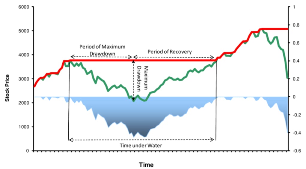
This event, the drawdown, creates an immediate and critical decision point. The operator must distinguish between two mutually exclusive states of the world:
State 1: Stochastic noise. The generative process of returns, G(xt|θ1), remains unchanged. The strategy is operating within its expected parameters, where θ1 includes a positive mean return (μ>0). It has simply encountered a statistically normal, albeit painful, period of adverse variance. This is an expected excursion into the left tail of the P&L distribution. The correct action is to do nothing. Intervening would be a catastrophic, unforced error—crystallizing a temporary loss, violating the strategy’s core assumptions, and missing the inevitable (if profitable) reversion to the mean.
State 2: Structural decay. The underlying market dynamics that generated the strategy’s alpha have fundamentally and irrevocably changed. The generative process has shifted from G(xt|θ1) to G(xt|θ2), where the new parameters θ2 imply a zero or negative mean return (μ≤0). The correct action is to intervene immediately, set position sizing to zero, and halt all new signal execution. Every new trade taken under this regime is a new, independent bet with a negative expected value.
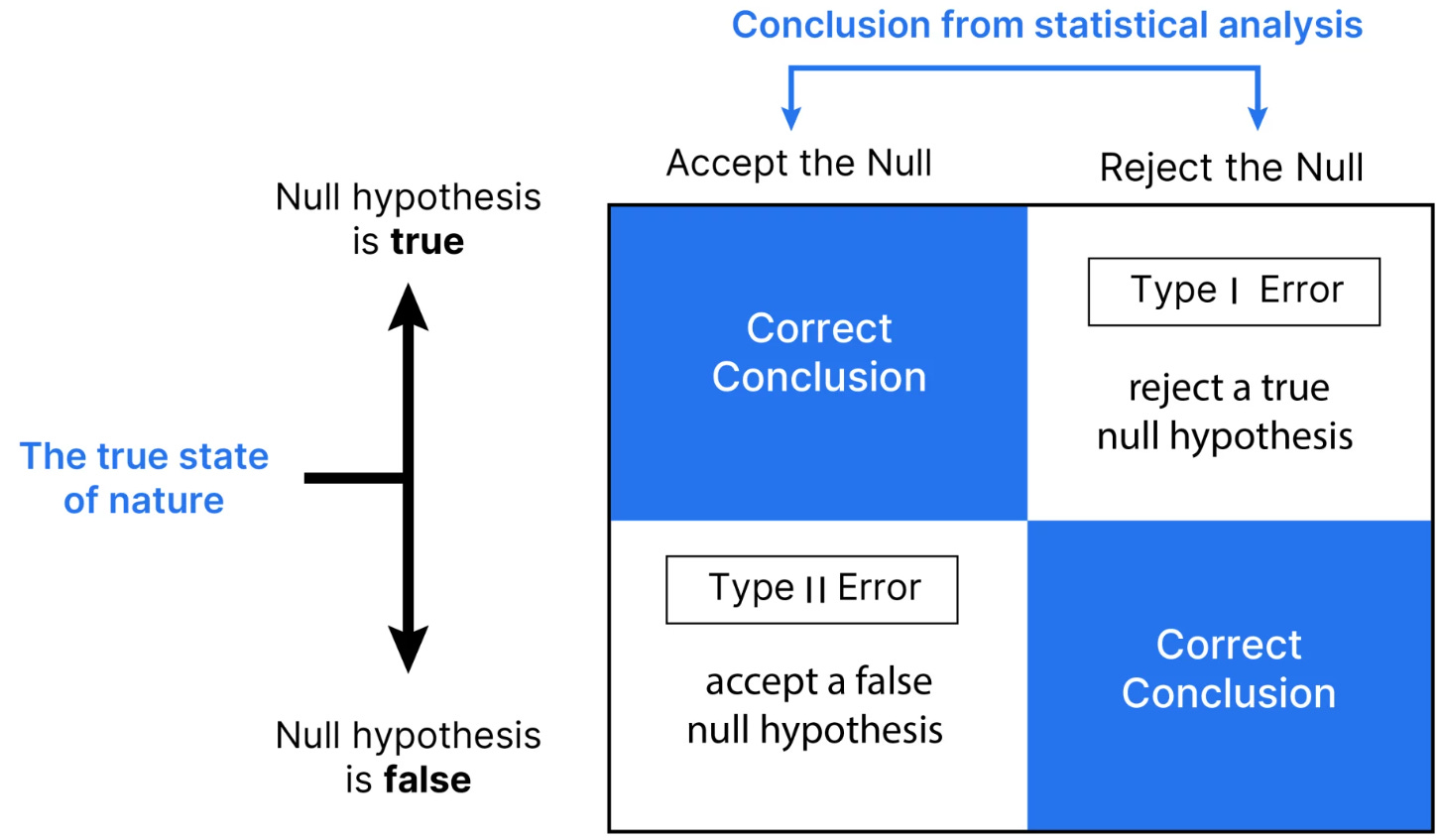
The cost of mis-identification is asymmetric and severe.
Cost of false positive (Type I error): Intervening on noise. You kill a profitable strategy. You crystallize a temporary loss and, more importantly, you miss the profitable recovery. This is a whipsaw. It’s an unforced error that destroys the geometric compounding of your capital. You have paid the cost of the drawdown without collecting the reward of the recovery.
Cost of false negative (Type II error): Failing to intervene on structural decay. This is an existential risk. It is the act of inertia—continuing to deploy capital into a statistically broken model. You are now systematically paying spread and slippage to execute a negative-expectancy strategy. You are not waiting for a recovery; you are actively digging a hole. This is how funds blow up. They transform a small, manageable drawdown from a broken strategy into a catastrophic, unrecoverable total loss.
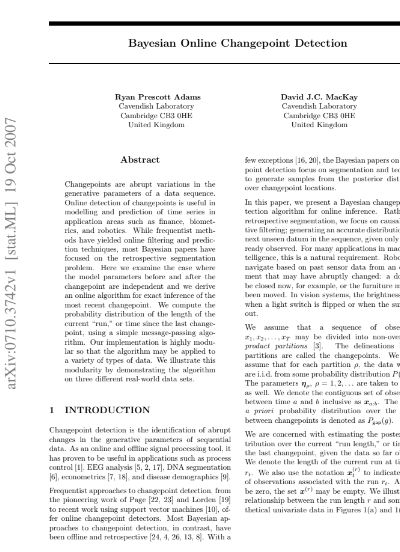
You can check here the original paper from which we have taken the implementation that we are going to develop:
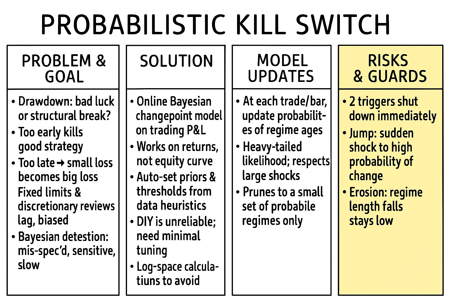
In this article we treat that decision explicitly as a probabilistic problem. Quants never observes “truth” directly; they only ever see a noisy, path–dependent P&L stream. Any rule that pretends otherwise—whether a hard 20% drawdown stop, a three-month underperformance review, or a hand-wavy committee meeting—is implicitly running a probabilistic model, usually a very bad one. The goal is to replace that collection of ad-hoc, inconsistent heuristics with a single, coherent decision rule that states, in clear numbers, how likely it is that the strategy has broken and what to do about it.
Legacy de-allocation frameworks tend to fall into two pathological extremes. On one side are purely heuristic rules:
Fixed drawdown limits, lookback Sharpe thresholds, rolling t-tests, or “if it feels wrong, turn it off.” These are simple to implement but blind to the true data-generating process; they confuse path properties of the equity curve with properties of the underlying returns.
On the other side are textbook Bayesian changepoint detectors, which assume idealised distributions, expose a large number of tunable hyperparameters, and often require full re-runs over the entire history. In theory they are elegant; in practice they are brittle, slow, and dangerously sensitive to mis-specification.
Risks and limitations of traditional and model-based de-allocation
Traditional risk management methods are woefully inadequate for this dilemma because they are deterministic, lagging, and non-probabilistic. They are relics of a discretionary world, not tools for a systematic one.
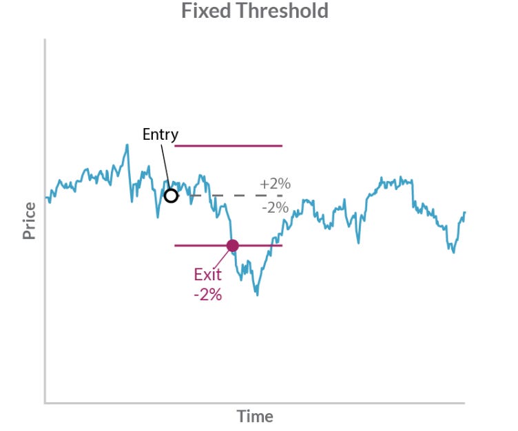
Fixed-threshold mechanisms: A 2% drawdown stop-loss is a primitive, lagging indicator. It is mathematically incoherent. It places a stop on the path (the cumulative P&L), not the process (the returns). It does not differentiate between a 2% loss from a single, sharp volatility shock (which may be a high-expectancy mean-reversion opportunity) and a 2% loss from a 1,000-trade slow bleed (which signifies certain alpha decay). This method functions by confirming a large loss has already occurred, guaranteeing the de-allocation is executed at the point of maximum pain. It is a purely reactive measure that carries no predictive power.

Discretionary intervention: A portfolio manager review is un-quantitative. It is a surrender of the entire systematic premise. It injects a portfolio of well-documented human biases directly into the risk model:
The sunk-cost fallacy: ”I’ve lost so much, I can’t stop now”.
Emotional attachment: ”This was my best strategy, it must come back”.
The gambler’s fallacy: ”It’s lost 10 times in a row, it must be due for a win”. This is not risk management; it is gambling.
An interesting alternative is a model-based approach, as described in the Adams & MacKay paper, Bayesian Online Changepoint Detection. However, this, too, is not a silver bullet. A naive implementation introduces its own, more sophisticated set of risks.
Model mis-specification risk: This is the primary and most dangerous risk. It is the assumption of an incorrect likelihood model for the data-generating process: Gaussian. Depending on your approach and type of model, the P&L could have different shapes. For example, a buy&hold approach will always see a fat-tailed event as a structural break, guaranteeing it will signal a false positive and trigger a whipsaw precisely when volatility expands.
Parameter sensitivity risk: A Bayesian model is, by definition, sensitive to its priors. This is a feature, not a bug, but it must be managed. The single most sensitive prior in BOCPD is the hazard rate, H, which is derived from the expected run length, λ. This parameter encodes our a priori belief about how often regimes should change.
A high hazard rate (low λ) creates a hyper-sensitive model. It has a weak prior on stability and will over-fit to noise, signaling changepoints constantly.
A low hazard rate (high λ) creates a sluggish, inertial model. It has a very strong prior on stability. It will require devastating, statistically overwhelming losses to overcome this prior. This model will commit the Type II error (failure to intervene) if not tuned correctly.
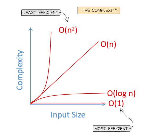
Computational complexity risk: An online algorithm must, by definition, run in linear time with respect to the data, O(T). A naive, textbook implementation of the BOCPD recursive update requires updating every possible past run length at every new time step. The total work to process a stream of length T is 1+2+...+T =T(T+1)/2. This is O(T2), or quadratic, complexity.

Probabilistic kill switch
The pivotal event driving our entire investigation is the structural break—the unknown moment in time, τ, when the generative parameters of our P&L stream, θ1, instantaneously shift to new parameters, θ2.
The problem is the financial trade-off between the cost of inertia (type II error / false negative) and the cost of whipsaw (type I error / false positive).
We need a de-allocation method—a kill switch—to solve this situation. A simple, fixed-ruleset cannot. We require a system that:
Operates in real-time, meaning O(K · T) complexity, where K<<T.
Is mathematically robust to the known statistical properties of financial data (i.e., leptokurtosis).
Is computationally tractable over thousand of data points, meaning it must be numerically stable.
Does not provide a binary “yes/no” answer, but rather a full posterior probability distribution of a changepoint.
This is the necessity. We must evolve our risk management from the primitive, deterministic question “How much have I lost?” to the key, probabilistic question:
What is the probability, given the data I’ve just seen, that the generative process of my returns has fundamentally broken?
We will now build this exact system from the ground up, based on the specific engineering and mathematical decisions in the bocpd_kill_switch method.
The idea is to feed a P&L stream into a BOCPD model and receive a kill signal. The challenge is that doing this correctly requires solving a series of non-trivial mathematical and engineering problems.
We will now analyze, in exhaustive detail, the seven critical technical challenges that must be solved.
Point 1: The non-stationarity fallacy
The first, and most common, failure in any time-series analysis is mis-handling the input data. A junior quant, looking at a beautiful cumulative P&L chart, will attempt to feed that chart directly into the model. This is a fatal mathematical error that invalidates the entire analysis before it even begins.
Our script’s first line of defense is not in the BOCPDRunner class, but in the analyze_pnl_stream wrapper function:
# THE SCRIPT’S FIRST ACTION:
returns = np.diff(cumulative_pnl, prepend=cumulative_pnl[0])
Why is this line non-negotiable? The answer is stationarity.
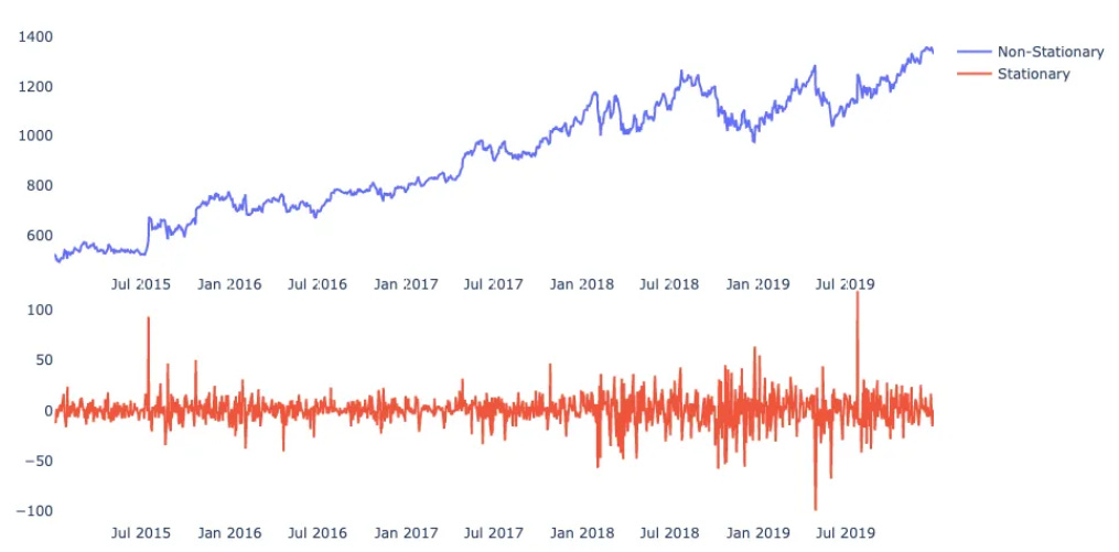
A stationary process is one whose statistical properties (mean, variance, autocorrelation) are constant over time. A cumulative P&L curve is, by definition, non-stationary. It is an integrated process of order 1, or I(1). It is, in simple terms, a random walk (with, one hopes, a positive drift).
Let’s be precise. The properties of a random walk, are:
Time-dependent mean: The expected value is a direct function of time. It is not constant.
\(E[PnL_t] = PnL_0 + \mu \cdot t\)Time-dependent variance: The variance also grows linearly with time. It is not constant.
\(Var(PnL_t) = \sigma^2 \cdot t\)
All standard statistical models, from ARIMA to GARCH to the generative model inside BOCPD, are built on the fundamental assumption that the data within a single regime is stationary (or can be modeled as such). They are designed to model a process, not an integrated path.
Modeling the cumulative P&L is like trying to measure the wind’s speed by only looking at a bird’s final displacement. You are measuring the accumulated result, not the generative process that created it. Any statistical measurement you take from the path (like its mean or variance) is a meaningless artifact of how long you measured, not a property of the process itself.
The returns, xt = PnLt - PnLt-1, are (or should be) our stationary, I(0) process. This is the generative process. The returns xt are the sequence of steps in the random walk. This process does have stable properties:
E[xt] = μ (constant)
Var(xt) = σ2 (constant)
This insight breaks a fundamental misconception. We are not detecting when the P&L curve flattens. That is a lagging, path-dependent observation. We are detecting when the statistical distribution of the steps changes.
The alpha of our strategy is the mean of this distribution, E[xt] = μ. When our strategy breaks, it means the generative process has shifted from P1(xt | μ1 > 0, σ1) to a new process P2(xt | μ2 > 0, σ2).
Therefore, the first critical action of our script is to differentiate the time series. All subsequent mathematics, every calculation, operates only on the returns array, xt.
Point 2: Automating priors with heuristics
The second major obstacle is that a Bayesian model requires priors. A naive BOCPD script would require a user to specify at least 10 different parameters: α0, β0, κ0, μ0 for the prior distribution, λ for the hazard rate, and various thresholds for the triggers.
A model with 10 knobs is not a tool but a research project. It creates a high risk of user error and data-dredging. The bocpd_kill_switch demonstrates a far more robust approach: parameter automation via heuristics.

The analyze_pnl_stream function derives its own parameters from the input data, making it a one-click diagnostic. This is the engineering wrapper that makes the science core usable.
# START OF PARAMETER AUTOMATION
T = len(returns)

# Heuristic 1: burn_in_period
burn_in_period = max(30, int(T * 0.15))

# Heuristic 2: expected_run_length (Lambda)
expected_run_length = max(burn_in_period + 10, int(T / 3.0))

# Heuristic 3: kill_threshold (Shock)
kill_threshold = 0.5 # Fixed: Risk Preference

# Heuristic 4: l_min (Erosion threshold)
l_min = max(15, int(expected_run_length * 0.25))

# Heuristic 5: m_consecutive
m_consecutive = max(5, int(l_min * 0.3))
# END OF AUTOMATION
Let’s analyze this logic in depth, as it is the secret sauce of the script.
Heuristic 1: burn_in_period
We set aside the first 15% of the data (with a 30-tick minimum) to learn the initial parameters of the first regime. This data is passed to the _init_priors function:
def _init_priors(self, burn_in_data):
    if len(burn_in_data) < 2:
        self.prior_m0 = 0.0
        var_guess = 0.01
    else:
        self.prior_m0 = np.mean(burn_in_data)
        var_guess = np.var(burn_in_data)

    self.prior_k0 = 1.0  # Low confidence in prior mean
    self.prior_a0 = 1.0  # Low confidence in prior variance

    if var_guess == 0: var_guess = 0.0001
    self.prior_b0 = var_guess * self.prior_a0 # Set prior scale
This is a critical step. Instead of forcing the user to guess the initial mean and variance of their strategy, we empirically measure them from the burn_in_data. The model is told:
Look at these first N ticks. This is what ‘normal’ looks like. Your job is to tell me when the data stops looking like this.
This makes the model data-driven and adaptive from the very first step. We set prior_k0 and prior_a0 to 1.0, which are uninformative priors, essentially telling the model, “Here’s our initial guess for the mean and variance, but don’t be too confident in it; learn from the data.”
Heuristic 2: expected_run_length (Lambda, λ)
This is the single most sensitive parameter in the entire model. It defines the hazard function, H, which is the a priori probability of a changepoint at any given step. For a constant hazard rate, as used here, H = 1/λ.
A low λ (e.g., 50) means a high hazard rate (H = 1/50 = 2%). We are telling the model “I expect regimes to break, on average, every 50 ticks.” The model will be hyper-sensitive, has a very weak prior on stability, and will over-fit to noise, signaling false changepoints.
A high λ (e.g., 2000) means a low hazard rate (H = 1/2000 = 0.05%). We are telling the model “I have a very strong belief that regimes are stable for a long time.” The model will be sluggish and inertial. It will require a catastrophic amount of evidence (i.e., massive losses) to overcome this strong prior.
Choosing λ is a dark magic. Our heuristic, expected_run_length = max(burn_in_period + 10, int(T / 3.0)), is a the choice here—so feel free to tune this part.
It states: “My agnostic, default assumption is that this P&L stream will contain approximately 3 distinct regimes.” This scales the model’s sensitivity to the length of the data being analyzed. A 3-year daily backtest (T=750) will get a λ ≈ 250, implying an average regime length of one year. A 1-day tick backtest (T=3000) will get a λ ≈ 1000, implying a new regime every ~1000 ticks. This is a far more robust starting point than a fixed number.
Heuristics 4 & 5: l_min and m_consecutive
These define our erosion trigger (which we will detail in Point 7). The key insight is that they are not fixed numbers. They are proportional to the expected_run_length.
l_min = 0.25 * expected_run_length: The erosion alarm sounds if the current regime’s expected lifespan (the ERL) falls below 25% of what we a priori defined as a normal lifespan.m_consecutive = 0.3 * l_min: The confirmation period—how long we wait in this “danger zone” before pulling the trigger—is also proportional, set to 30% of the danger threshold itself.
This proportionality makes the trigger time-scale invariant. An Expected Run Length (ERL) of 25 on a swing-trading strategy (where λ=100) is just as alarming as an ERL of 250 on an HFT strategy (where λ=1000).
Point 3: The engine (the recursive update)
Now we enter the core of the BOCPDRunner class: the update function. This is the mathematical engine that propogates our beliefs forward in time.
The model maintains a vector of probabilities, Rt, whereRt(i) is the probability that the current run length rt is equal to i.
To get the next step’s probability vector, Rt+1, we must compute two components for every possible previous run length i:
The growth probability: The probability that the regime continues. The run length rt+1 will be i+1.
\(P(\text{Growth}) = P(r_t = i | x_{1:t}) \cdot P(x_{t+1} | x_{t-i:t}) \cdot (1-H(i))\)P(rt= i | x1:t) is our prior belief from the last step (the value of
log_R_t[i]).P(xt+1 | ...) is the predictive likelihood: How likely is the new data point xt+1 given the data we’ve seen in this i-length run? This is the output of
_log_student_t_predictive.(1-H(i)) is the prior probability of no changepoint (our
log_neg_hazard).
The changepoint probability: The probability that the regime breaks. The new run length rt+1 will be 0.
\(P(\text{Change}) = P(r_t = i | x_{1:t}) \cdot P(x_{t+1} | x_{t-i:t}) \cdot H(i)\)H(i) is the hazard rate, the prior probability of a changepoint (our
log_hazard).
The total probability of a changepoint, P(rt+1 = 0), is the sum of all changepoint probabilities from all possible previous run lengths:
The new probability vector Rt+1 is then formed by:
Finally, we must normalize Rt+1so it sums to 1. This trellis of calculations, where each step’s probabilities are passed to the next, is the core of the algorithm. However, a naive implementation of this math will not work.
Point 4: Numerical stability via log-space
Why is the bocpd_kill_switch script filled with np.log, np.exp, gammaln, and logsumexp? Why not just multiply the probabilities as defined in Point 3?
Answer: Numerical underflow.
Probabilities are small numbers, often < 1.0. Multiplying many small numbers together creates astronomically small numbers.
P(seq) = 0.1 x 0.5 x 0.2 x 0.1 = 0.001
After just 100 ticks, a typical sequence probability might be 0.1100 = 10-100.
A standard 64-bit floating-point number in Python (float) cannot represent this. The machine precision bottoms out (around 10-308), and the number is rounded to 0.0. The algorithm breaks. The entire probability vector Rt becomes [0.0, 0.0, ..., 0.0]. This isn’t a minor bug but a complete failure of the algorithm.
The solution: We perform all calculations in log-space.
By applying the logarithm, we transform our numbers from the probability domain [0, 1] to the log-probability domain [-inf, 0]. This conversion exploits two key mathematical identities:
Multiplication becomes addition: log(A·B)=log(A)+log(B)
This is computationally fast and numerically stable. Adding log(10-100) and log(10-50) gives -100·log(10) - 50·log(10) = -230 - 115 = -345. This is a perfectly reasonablefloatfor a computer to store.Addition becomes
logsumexp: log(A + B) = log(elog A + elog B)
This is the tricky part. We can’t just add log-probabilities. Thelogsumexpfunction is a numerically careful way to compute this by factoring out the maximum value:\(\log(A+B) = \log(e^{\log A - \log M} + e^{\log B - \log M}) + \log M, \text{ where } \log M = \max(\log A, \log B)\)
Now, look at the actual implementation in the update function and compare it to the math in Point 3.
The part of the code that is in charged of this is:
# log_R_t is log(P(r_t=i))
# log_pred_probs is log(P(x_{t+1} | ...))
# self.log_neg_hazard is log(1 - H(i))
# self.log_hazard is log(H(i))

# 1. Growth (Multiplication -> Addition)
log_growth_probs = self.log_R_t + log_pred_probs + self.log_neg_hazard

# 2. Change (Sum of Products -> logsumexp of sums)
log_cp_prob = logsumexp(self.log_R_t + log_pred_probs + self.log_hazard)

# ...

# 5. Normalization (Division -> Subtraction)
# P(r_t) / sum(P(r_t)) -> log(P(r_t)) - log(sum(P(r_t)))
# log(sum(P(r_t))) = log(sum(exp(log(P(r_t))))) = logsumexp(log_R_t)
log_norm_const = logsumexp(new_log_R_t)
self.log_R_t = new_log_R_t - log_norm_const
This is a direct translation of the recursive Bayesian update into a numerically stable form. This section is not a minor detail. This log-space implementation is the only thing that allows the algorithm to run for more than a few hundred ticks. It is the difference between a textbook theory and a production-grade tool.
Point 5: The N-IG / Student-t likelihood
We have an engine. Now we must feed it. The most important part of the engine is the log_pred_probs—the predictive likelihood function P(xt+1|xt-1:t). This function answers the question: How likely is this new data point, given the regime we are assuming we’re in?
The second, and equally fatal, mistake a quant can make is to assume a Gaussian (Normal) distribution for returns.
Financial returns are not Gaussian. They are leptokurtic. They have fat tails and excess kurtosis. A 4-sigma event, which a Gaussian model treats as a 1-in-3.5-million impossibility (P≈3x10⁻⁵), is something a financial market produces every few years, or even months. It is not an impossible event; it is an expected (if infrequent) feature of the landscape.
If you use a Gaussian likelihood (scipy.stats.norm.pdf):
A 4-sigma return xt occurs.
The model calculates its likelihood: P(xt | Gaussian regime)≈3x10⁻⁵.
In log-space, this is a massive penalty: log(10-5) ≈ -11.5.
This huge negative number is added to all
log_growth_probs, effectively killing them.The model concludes it is impossible for xt to have come from the old regime. P(xt+1=0) spikes to ~100%.
The model signals a false positive. It has mistaken a normal (but volatile) market day for a structural break.
We must use a likelihood model that expects fat tails. Our script does this using a Normal-Inverse-Gamma (N-IG) prior.
This is a 4-parameter conjugate prior for a Gaussian process with both unknown mean AND unknown variance. This is key. We are not just modeling the mean (our alpha); we are modeling the mean, the variance (our risk), and our uncertainty about both.
The N-IG prior is defined by four hyperparameters (which we set in _init_priors):
prior_m0(μ0): The prior mean.prior_k0(κ0): Our confidence in the prior mean.prior_a0(α0): The shape of the prior variance (an Inverse-Gamma dist).prior_b0(β0): The scale of the prior variance.
The mathematical magic is this: when you have a Gaussian likelihood with an N-IG prior, the posterior predictive distribution (the distribution of a new data point, after integrating out all uncertainty about the unknown μ and σ2) is not a Gaussian. It is a Student-t distribution.

The _log_student_t_predictive function is the log-PDF of this distribution:
def _log_student_t_predictive(self, data_point):
    # ...
    # df = degrees of freedom
    df = 2 * self.alphas
    loc = self.mus
    scale_sq = self.betas * (self.kappas + 1) / ((self.alphas * self.kappas) + epsilon)
    # ...
    log_prob = (gammaln(df / 2.0 + 0.5) -
                gammaln(df / 2.0) -
                0.5 * np.log(df * np.pi * scale_sq) -
                (df / 2.0 + 0.5) * np.log(1.0 + (data_point - loc)**2 / (df * scale_sq)))

    return log_prob
Notice that the degrees of freedom df are not fixed, but are derived from self.alphas, which is learned from the data. As the model sees more data in a run (and self.alphas grows), the df increases, and the Student-t distribution slowly converges to a Gaussian. This is mathematically beautiful. It’s a model that says
“When I have little data (low
df), I assume fat tails. As I gain confidence from more data (highdf), I will tighten my assumptions and converge towards a Normal distribution.”
When this model (with a low df, e.g., df=4) sees a 4-sigma event, the t-distribution assigns it a low, but not impossible, probability (e.g., P=0.01). The log-likelihood is log(0.01)≈-4.6.
Gaussian penalty: -11.5
Student-t penalty: -4.6
The t-distribution’s penalty is far smaller. The model thinks:
“That was unlikely, but plausible. I will reduce my belief in this regime, but I will not discard it.”
This prevents the false positive. The N-IG model is updated analytically in O(1) time, which is what the update function does:
# 6. Update sufficient statistics for each run length
new_alphas = self.alphas + 0.5
new_betas = self.betas + (self.kappas * (data_point - self.mus)**2) / (2.0 * (self.kappas + 1.0))
new_kappas = self.kappas + 1.0
new_mus = (self.kappas * self.mus + data_point) / new_kappas
This is the conjugate update. It is the learning part of the algorithm.
new_kappasandnew_alphasgrow with each data point, increasing our confidence (dfgoes up).new_musbecomes a weighted average of the prior mean and the data mean.new_betasaccumulates the sum of squared errors, updating our variance estimate.
Point 6: State-space pruning
We have a robust, numerically stable model. Now we have a new problem: computational complexity.
Let’s follow the logic:
At time t=100, our
log_R_tvector has 101 elements (for xt=0 to xt=100). We also have 101 sets of N-IG parameters (alphas,betas,kappas,mus).To compute
log_R_tat t=101, we must update all 101 hypotheses.At time t=T, our
log_R_tvector has T+1 elements. We must run T+1 updates.The total work to process a stream of length T is 1 + 2 + 3 + ... + T = T(T+1)/2.
The complexity is O(T2), or quadratic.
This is a catastrophic failure for a high-frequency context. A 10,000-tick backtest would require ~50,000,000 operations. A 100,000-tick backtest would require ~5,000,000,000 operations. The algorithm does not scale. It is not online. It’s not just a speed problem; it’s a memory problem. We’d have to store T copies of our 4 state-space vectors, an O(T2) memory footprint.
If we are at t=1000, what is the probability that the true run length is xt=5 It is astronomically small. What about xt=998? Also astronomically small. The true posterior probability mass P(xt| xt:1) is clustered around a few, plausible run lengths. We do not need to waste CPU cycles and RAM updating hypotheses that have a 10-50 probability of being correct.
Our script implements this optimization aggressively in the update function:
# 8. Pruning: Discard states with vanishingly small probability
keep_indices = np.where(self.log_R_t > self.prune_threshold)[0]

if len(keep_indices) == 0:
     # Failsafe: if pruning is too aggressive, keep at least the most likely state
    keep_indices = np.array([np.argmax(self.log_R_t)])

self.log_R_t = self.log_R_t[keep_indices]
self.alphas = self.alphas[keep_indices]
self.betas = self.betas[keep_indices]
self.kappas = self.kappas[keep_indices]
self.mus = self.mus[keep_indices]
The self.prune_threshold is set to -10.0. Since we are in log-space, this means log(P) = -10 ⇒ P = e-10 ≈ 0.000045.
We are aggressively culling any run-length hypothesis whose posterior probability falls below 0.0045%.
The result is that the number of active hypotheses, K (the length of self.log_R_t), does not grow to T. It stays at a small, roughly constant size, K << T (e.g., K ≈ 100-200, regardless of whether T=1,000 or T=10,000,000).
This optimization reduces the computational complexity. This is linear time complexity. The memory footprint is also reduced from O(T2) to O(K·T). This is what makes the algorithm “online” and computationally feasible for real-world, high-frequency data streams. The prune_threshold is a trade-off between accuracy and speed, but at -10.0, the amount of discarded probability mass is negligible.

Point 7: The dual-trigger system
We have a robust, stable, and fast probabilistic model. It does not give us a yes/no answer. It gives us a full probability distribution log_R_t at every tick.
Now, we must make a decision. How do we turn this rich, complex distribution into a single, binary kill signal for our execution engine?
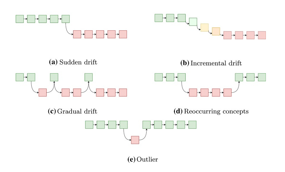
A strategy can die in two distinct ways. A robust kill switch must detect both.
Failure mode 1: The shock: This is a sudden, catastrophic event. A deal breaks, an FOMC announcement surprises, a flash crash occurs. The P&L gaps down violently. The return xt is a single, massive, deeply negative outlier.
Failure Mode 2: The erosion: This is a slow, painful bleed. The alpha edge slowly drifts from
+0.1to-0.01. Competitors have crowded the trade, or the market feature has been arbitraged away. No single return xt is catastrophic, but the sequence of returns is consistently poor, and the P&L drifts to zero (or negative).
Our script implements a dedicated trigger for each of these modes.
Trigger 1: The shock (kill_signals_shock)
# Rule 1: Shock Kill
if cp > kill_threshold:
    kill_signals_shock[t] = True
This is the simple, direct trigger. cp is the changepoint probability, P(xt| xt:1). This is the value we calculated as log_cp_prob and converted with np.exp(). Our kill_threshold is hard-coded (via our heuristic) to 0.5.
The logic is simple, elegant, and defensible: If it is more likely than not (P > 50%) that the regime broke on this exact tick, we de-allocate immediately. This is a pure, Bayesian decision-theory threshold.
This trigger will catch the outlier. The _log_student_t_predictive function will see a catastrophically unlikely return (e.g., -10 sigma). It will assign a massive log-probability penalty to all growing regimes. The only hypothesis that doesn’t get this penalty is the new one which starts from the fresh priors. As a result, all probability mass in the logsumexp calculation will flood to log_cp_prob, pushing P(xt=0) above 50% and firing the trigger.
Trigger 2: The erosion (kill_signals_erosion)
grace_period = burn_in_period + l_min
if exp_rl < l_min and t > grace_period:
    erosion_counter += 1
else:
    erosion_counter = 0 # Reset counter

if erosion_counter >= m_consecutive:
    # ... fire signal
This is the far more subtle and, frankly, more important trigger. In an erosion scenario, the shock trigger will never fire. No single return xt is bad enough to cross the 50% threshold.
Instead, the model just gets confused. The returns are all slightly negative or noisy. They don’t look like the great regime from the burn-in, but they aren’t terrible either. The model thinks: This doesn’t look like regime 1... but it’s not a clear-cut shock. Maybe a new, mediocre regime started 10 ticks ago? Or 5 ticks ago? Or 20 ticks ago?
In this state of confusion, the posterior probability mass in log_R_t scatters. It doesn’t commit to the long-running regime, but it also doesn’t commit to rt=0. The mass spreads out over many small, recent run-length hypotheses.
When this happens, the expected run length (exp_rl)—which is the probability-weighted average of all active run lengths (np.sum(np.exp(self.log_R_t) * active_run_lengths))—collapses. It won’t go to 0, but it will drop from (e.g.) 150 to a low number, like 20.
This trigger’s logic is:
If the ERL (
exp_rl) drops below our auto-calculated pain threshold (l_min) and stays there form_consecutiveticks, we have confirmation of structural erosion. The model is admitting it cannot find a stable, long-running regime. Kill the strategy.
The grace_period is a critical failsafe. It prevents this trigger from firing right after the burn_in, when the ERL is supposed to be low (since it’s just starting to grow from 0). This prevents an immediate false positive.
This dual-trigger system is a robust decision-making framework that handles multiple, distinct failure archetypes.
Alright! Time to test the method, let’s see what this thing have for us:
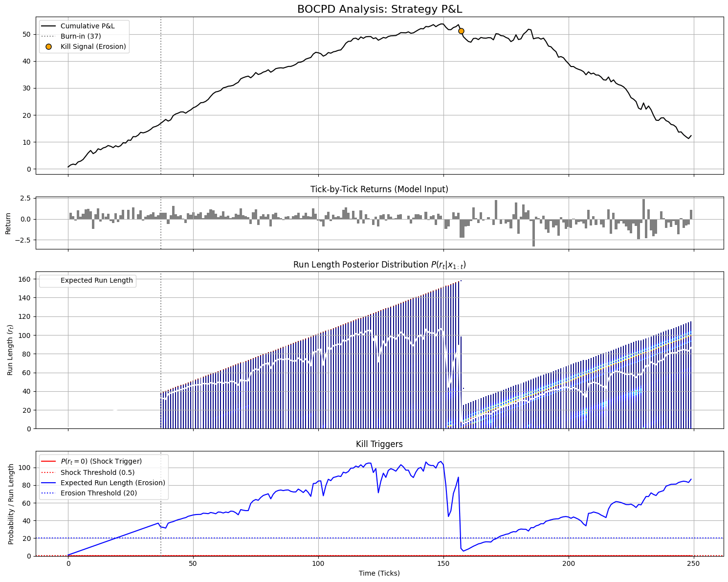
After a short burn-in period (grey dashed line at tick 37) the equity curve climbs steadily, peaks around tick 150, and then starts to erode; the orange dot marks the time where the system issues a kill signal.
The second panel contains the tick-by-tick returns that feed the model. The third panel shows, for every time step, the posterior distribution of the run length (how long the current regime has lasted). In the profitable phase the expected run length (white line) grows almost linearly, indicating a stable regime, and then suddenly collapses when the behaviour changes. The bottom panel translates this into kill triggers.

Until next time—may your trades be as precise as a masterstroke, your signals as clear as dawn’s first light, and your returns as bold as a bull’s charge. Navigate the markets with poise, resilience, and an unshakable edge 🚀
PS: I have included the Intel Reports from the MarketOps section in the Substack app, do you prefer it coninuous hided?
This is an invitation-only access to our QUANT COMMUNITY, so we verify numbers to avoid spammers and scammers. Feel free to join or decline at any time. Tap the WhatsApp icon below to join

Appendix
Full script:
import numpy as np
import matplotlib.pyplot as plt
from scipy.special import logsumexp, gammaln

class BOCPDRunner:
    “”“
    A robust, log-space implementation of Bayesian Online Changepoint
    Detection (BOCPD) using a Normal-Inverse-Gamma conjugate prior,
    which results in a Student-t posterior predictive distribution.

    This class is designed to be fed one data point at a time.
    “”“

    def __init__(self, hazard_lambda=250.0, prune_threshold_log_prob=-10.0):
        “”“
        Initializes the BOCPD runner.

        Args:
            hazard_lambda (float): The expected run length of a regime.
                                   This defines the hazard rate (1/lambda).
            prune_threshold_log_prob (float): Log-probability threshold
                                              to prune state space for speed.
        “”“
        self.hazard_lambda = hazard_lambda
        self.log_hazard = np.log(1.0 / self.hazard_lambda)
        self.log_neg_hazard = np.log(1.0 - (1.0 / self.hazard_lambda))
        self.prune_threshold = prune_threshold_log_prob

        # These will be set by _init_priors
        self.prior_a0 = None  # Prior Alpha (shape) for Inv-Gamma
        self.prior_b0 = None  # Prior Beta (scale) for Inv-Gamma
        self.prior_k0 = None  # Prior Kappa (confidence) for Normal
        self.prior_m0 = None  # Prior Mu (mean) for Normal

        # These are the live state vectors, storing beliefs for all
        # possible run lengths. We initialize with a single run of length 0.
        self.log_R_t = np.array([0.0])  # Log-prob of run length. R[i] = P(r_t = i)
        self.alphas = np.array([])     # Run-length specific Alphas
        self.betas = np.array([])      # Run-length specific Betas
        self.kappas = np.array([])     # Run-length specific Kappas
        self.mus = np.array([])        # Run-length specific Mus

    def _init_priors(self, burn_in_data):
        “”“
        “Automatizes” the priors based on a burn-in data segment.

        Args:
            burn_in_data (np.array): Initial data points to set priors.
        “”“
        # Use empirical mean and variance from burn-in
        # Handle case where burn_in_data might be empty or too small
        if len(burn_in_data) < 2:
             # Default to simple priors if burn-in is insufficient
            self.prior_m0 = 0.0
            var_guess = 0.01
        else:
            self.prior_m0 = np.mean(burn_in_data)
            var_guess = np.var(burn_in_data)

        self.prior_k0 = 1.0  # Low confidence in prior mean

        self.prior_a0 = 1.0  # Low confidence in prior variance

        # Handle zero variance in burn-in (e.g., flat P&L)
        if var_guess == 0:
            var_guess = 0.0001
        self.prior_b0 = var_guess * self.prior_a0 # Set prior scale

        print(f”Priors Initialized: Mu={self.prior_m0:.4f}, “
              f”Var_Guess={var_guess:.4f}”)

        # Initialize live state vectors with these priors
        self.alphas = np.array([self.prior_a0])
        self.betas = np.array([self.prior_b0])
        self.kappas = np.array([self.prior_k0])
        self.mus = np.array([self.prior_m0])

    def _log_student_t_predictive(self, data_point):
        “”“
        Calculates the log-probability of the data point under the
        posterior predictive (Student-t) for all active run lengths.

        This is the core of the (N-IG -> Student-t) model.

        Args:
            data_point (float): The new data point (a single return).

        Returns:
            np.array: An array of log-probabilities, one for each
                      active run length.
        “”“
        # Handle potential empty state vectors during initialization
        if len(self.alphas) == 0:
            return np.array([])

        # This is the log-pdf of the Student-t distribution
        # log P(x | r_t, x_{1:t-1})
        df = 2 * self.alphas
        loc = self.mus

        # Add small epsilon to avoid division by zero if alphas or kappas are zero
        epsilon = 1e-10
        scale_sq = self.betas * (self.kappas + 1) / ((self.alphas * self.kappas) + epsilon)

        # Avoid invalid values in log (e.g., scale_sq <= 0)
        scale_sq = np.maximum(scale_sq, epsilon)

        # Gammaln is log(Gamma(x))
        log_prob = (gammaln(df / 2.0 + 0.5) -
                    gammaln(df / 2.0) -
                    0.5 * np.log(df * np.pi * scale_sq) -
                    (df / 2.0 + 0.5) * np.log(1.0 + (data_point - loc)**2 / (df * scale_sq)))

        return log_prob

    def update(self, data_point):
        “”“
        Processes a single new data point and updates all internal states.

        Args:
            data_point (float): The new data point (a single return).

        Returns:
            tuple: (changepoint_prob, expected_run_length)
        “”“
        # 1. Calculate log-predictive probability for each run length
        log_pred_probs = self._log_student_t_predictive(data_point)

        # Handle empty log_R_t during first step
        if len(self.log_R_t) == 0:
            log_growth_probs = np.array([])
        else:
            # 2. Calculate “Growth” probabilities (log-space)
            # P(r_t = r_{t-1} + 1 | x_{1:t})
            log_growth_probs = self.log_R_t + log_pred_probs + self.log_neg_hazard

        # 3. Calculate “Changepoint” probability (log-space)
        # P(r_t = 0 | x_{1:t})
        # This is the “kill trigger” probability
        if len(self.log_R_t) == 0:
            log_cp_prob = np.log(1.0) # On first step, changepoint is 100%
        else:
            log_cp_prob = logsumexp(self.log_R_t + log_pred_probs + self.log_hazard)

        # 4. Form new run-length distribution
        # We shift all growth probs one step to the right
        # and insert the new changepoint prob at r_t = 0
        new_log_R_t = np.insert(log_growth_probs, 0, log_cp_prob)

        # 5. Normalize the distribution
        log_norm_const = logsumexp(new_log_R_t)
        self.log_R_t = new_log_R_t - log_norm_const

        # 6. Update sufficient statistics for each run length
        # Standard N-IG conjugate update rules
        if len(self.alphas) == 0:
            new_alphas = np.array([])
            new_betas = np.array([])
            new_kappas = np.array([])
            new_mus = np.array([])
        else:
            new_alphas = self.alphas + 0.5
            new_betas = self.betas + (self.kappas * (data_point - self.mus)**2) / (2.0 * (self.kappas + 1.0))
            new_kappas = self.kappas + 1.0
            new_mus = (self.kappas * self.mus + data_point) / new_kappas

        # 7. Prepend the “new run” (r_t=0) priors to the stats
        self.alphas = np.insert(new_alphas, 0, self.prior_a0)
        self.betas = np.insert(new_betas, 0, self.prior_b0)
        self.kappas = np.insert(new_kappas, 0, self.prior_k0)
        self.mus = np.insert(new_mus, 0, self.prior_m0)

        # 8. Pruning: Discard states with vanishingly small probability
        keep_indices = np.where(self.log_R_t > self.prune_threshold)[0]

        if len(keep_indices) == 0:
             # Failsafe: if pruning is too aggressive, keep at least the most likely state
            keep_indices = np.array([np.argmax(self.log_R_t)])

        self.log_R_t = self.log_R_t[keep_indices]
        self.alphas = self.alphas[keep_indices]
        self.betas = self.betas[keep_indices]
        self.kappas = self.kappas[keep_indices]
        self.mus = self.mus[keep_indices]

        # Return metrics
        changepoint_prob = np.exp(log_cp_prob)
        # Note: ‘keep_indices’ might not start from 0 after pruning
        # We need to map back to actual run lengths
        active_run_lengths = keep_indices
        if len(active_run_lengths) > 0 and len(self.log_R_t) > 0:
            expected_run_length = np.sum(np.exp(self.log_R_t) * active_run_lengths)
        else:
            expected_run_length = 0

        return changepoint_prob, expected_run_length, self.log_R_t.copy(), keep_indices.copy()

def analyze_pnl_stream(cumulative_pnl):
    “”“
    Main wrapper function to run BOCPD on a cumulative P&L stream.
    ¡Todos los parámetros ahora son automáticos!

    Args:
        cumulative_pnl (np.array): The input array of cumulative P&L.
    “”“

    # 1. Convert cumulative P&L to returns
    if len(cumulative_pnl) < 2:
        print(”Error: P&L stream is too short.”)
        return
    returns = np.diff(cumulative_pnl, prepend=cumulative_pnl[0])
    T = len(returns)

    if T < 50:
        print(f”Error: Data is too short (T={T}). Need at least 50 data points for auto-analysis.”)
        return

    # Heuristic 1: burn_in_period
    burn_in_period = max(30, int(T * 0.15))

    # Heuristic 2: expected_run_length (Lambda)
    expected_run_length = max(burn_in_period + 10, int(T / 3.0))

    # Heuristic 3: kill_threshold (Shock)
    kill_threshold = 0.5

    # Heuristic 4: l_min (Erosion threshold)
    l_min = max(15, int(expected_run_length * 0.25))

    # Heuristic 5: m_consecutive
    m_consecutive = max(5, int(l_min * 0.3))

    print(”--- Análisis BOCPD con Parámetros Automáticos ---”)
    print(f”Total Ticks (T):       {T}”)
    print(f”Burn-in Period:        {burn_in_period}”)
    print(f”Expected Run Length:   {expected_run_length}”)
    print(f”Shock Kill Threshold:  {kill_threshold}”)
    print(f”Erosion Kill (l_min):  {l_min}”)
    print(f”Erosion Ticks (m):     {m_consecutive}”)
    print(”-------------------------------------------------”)

    # 2. Initialize Model
    model = BOCPDRunner(hazard_lambda=float(expected_run_length))

    # 3. “Automatize” Priors
    burn_in_data = returns[:burn_in_period]
    model._init_priors(burn_in_data)

    # 4. Storage for results
    cp_probs = np.zeros(T)
    exp_rls = np.zeros(T)
    kill_signals_shock = np.zeros(T, dtype=bool)
    kill_signals_erosion = np.zeros(T, dtype=bool)

    # Trellis plot storage
    run_length_distributions = []

    # 5. Run Online Loop
    print(f”Running BOCPD from t=0 to t={T}...”)
    erosion_counter = 0

    # Run loop from t=0, but only start *updating* after burn-in
    for t in range(T):
        if t < burn_in_period:
            # During burn-in, just feed data to prime the first run length
            # We don’t record these as “real” triggers
            cp, exp_rl, log_R, indices = model.update(returns[t])

            cp_probs[t] = 0.0 # No triggers during burn-in
            exp_rls[t] = t + 1
            run_length_distributions.append(
                (np.array([t]), np.array([0.0])) # (indices, log_probs)
            )
            continue

        # This is the core update step post-burn-in
        cp, exp_rl, log_R, indices = model.update(returns[t])

        cp_probs[t] = cp
        exp_rls[t] = exp_rl
        run_length_distributions.append((indices, log_R))

        # Apply Kill Rules
        # Rule 1: Shock Kill
        if cp > kill_threshold:
            kill_signals_shock[t] = True

        # Rule 2: Erosion Kill
        # Don’t check for erosion until the model has had a chance
        # to build up a run length (l_min ticks after burn_in)
        grace_period = burn_in_period + l_min
        if exp_rl < l_min and t > grace_period:
            erosion_counter += 1
        else:
            erosion_counter = 0 # Reset counter

        if erosion_counter >= m_consecutive:
            # Fire signal for all days in the erosion period
            for i in range(m_consecutive):
                kill_signals_erosion[t-i] = True

    print(”Analysis Complete.”)

    # 6. Plotting
    plot_results(cumulative_pnl, returns, cp_probs, exp_rls,
                 kill_signals_shock, kill_signals_erosion,
                 run_length_distributions, T, burn_in_period,
                 kill_threshold, l_min) # Pass l_min for plotting

def plot_results(cum_pnl, returns, cp_probs, exp_rls,
                 kills_shock, kills_erosion,
                 rl_dists, T, burn_in, kill_thresh, l_min):
    “”“Helper function to generate the final plots.”“”

    fig, (ax0, ax1, ax2, ax3) = plt.subplots(4, 1, figsize=(15, 12),
                                         sharex=True,
                                         gridspec_kw={’height_ratios’: [3, 1, 3, 2]})

    # Plot 1: Cumulative P&L
    ax0.plot(cum_pnl, ‘k-’, label=’Cumulative P&L’)
    ax0.set_title(’BOCPD Analysis: Strategy P&L’, fontsize=16)
    ax0.axvline(burn_in, color=’gray’, linestyle=’:’, label=f’Burn-in ({burn_in})’)

    # Plot kill signals on P&L
    shock_points = np.where(kills_shock)[0]
    erosion_points = np.where(kills_erosion)[0]
    if len(shock_points) > 0:
        # Plot only the first point of each contiguous block
        shock_starts = shock_points[np.diff(shock_points, prepend=-1) > 1]
        ax0.plot(shock_starts, cum_pnl[shock_starts], ‘rv’,
                 markersize=8, label=’Kill Signal (Shock)’)
    if len(erosion_points) > 0:
        # Plot only the first point of each contiguous block
        erosion_starts = erosion_points[np.diff(erosion_points, prepend=-1) > 1]
        ax0.plot(erosion_starts, cum_pnl[erosion_starts], ‘o’,
                 mfc=’orange’, mec=’k’, markersize=8, label=’Kill Signal (Erosion)’)
    ax0.legend(loc=’upper left’)
    ax0.grid(True)

    # Plot 2: Tick-by-Tick Returns
    ax1.bar(range(T), returns, color=’gray’, width=1.0)
    ax1.set_title(’Tick-by-Tick Returns (Model Input)’)
    ax1.axvline(burn_in, color=’gray’, linestyle=’:’)
    ax1.set_ylabel(’Return’)
    ax1.grid(True)

    # Plot 3: Run Length Distribution (Trellis)
    ax2.set_title(’Run Length Posterior Distribution $P(r_t | x_{1:t})$’)
    ax2.set_ylabel(’Run Length ($r_t$)’)
    ax2.grid(True)

    # Create the trellis plot from our stored distributions
    max_run_length = 0
    for t in range(burn_in, T):
        indices, log_R = rl_dists[t]
        if len(indices) == 0: continue

        # Convert log-probs to probabilities and normalize for color
        probs = np.exp(log_R - log_R.max()) # Normalize for color
        colors = plt.cm.jet(probs)
        ax2.scatter(np.full_like(indices, t), indices, c=colors,
                    s=2, marker=’s’, lw=0)

        if len(indices) > 0:
            max_run_length = max(max_run_length, indices.max())

    ax2.plot(exp_rls, ‘w-’, lw=2, label=’Expected Run Length’)
    ax2.axvline(burn_in, color=’gray’, linestyle=’:’)
    ax2.legend(loc=’upper left’)
    ax2.set_ylim(0, max(max_run_length + 10, l_min + 10)) # Dynamic ylim

    # Plot 4: Kill Trigger Probabilities
    ax3.plot(cp_probs, ‘r-’, label=’$P(r_t = 0)$ (Shock Trigger)’)
    ax3.axhline(kill_thresh, color=’r’, linestyle=’:’,
                label=f’Shock Threshold ({kill_thresh})’)

    # Plot Erosion trigger
    ax3.plot(exp_rls, ‘b-’, label=’Expected Run Length (Erosion)’)
    ax3.axhline(l_min, color=’b’, linestyle=’:’,
                label=f’Erosion Threshold ({l_min})’)

    ax3.set_title(’Kill Triggers’)
    ax3.set_xlabel(’Time (Ticks)’)
    ax3.set_ylabel(’Probability / Run Length’)
    ax3.axvline(burn_in, color=’gray’, linestyle=’:’)

    # Dynamic ylim for this plot
    max_y_cp = np.max(cp_probs)
    max_y_erl = np.max(exp_rls[burn_in:]) if burn_in < T else l_min
    max_y = max(max_y_cp, max_y_erl, l_min, kill_thresh)

    ax3.set_ylim(-0.05, max_y * 1.1 + 1)

    ax3.legend(loc=’upper left’)
    ax3.grid(True)

    plt.tight_layout()
    plt.show()


if __name__ == “__main__”:

    # 1. Create a more dramatic simulation to show triggers firing
    np.random.seed(482)
    T_good = 150
    T_bad = 100

    # Regime 1: Good Sharpe (Mean 0.3, Std 0.5)
    returns_good = np.random.normal(0.3, 0.5, T_good)

    # Regime 2: BAD (Mean -0.4, Std 1.0) -> Mean reversal AND vol explosion
    returns_bad = np.random.normal(-0.4, 1.0, T_bad)

    returns_stream = np.concatenate([returns_good, returns_bad])

    # Create cumulative P&L from returns (this is the user’s input)
    pnl_stream = np.cumsum(returns_stream)

    print(”Starting BOCPD Auto-Analysis”)

    # 2. Run the analysis
    analyze_pnl_stream(pnl_stream)

    print(”Analysis Finished”)