[WITH CODE] Optimization: Robust protocol

A robust protocol for: 1 variable + 1 model + 1 parameter

---

Table of contents:

1. Introduction.

2. Performance vs. Robustness.

3. Risks and model limitations.

4. Parameter selection without a foundation.

5. Robust optimization protocol.

   1. Problem statement and design goals.

   2. CV for dependent data.

   3. Control-group testing on each split.

   4. Split-level aggregation and the conditional superiority probability.

   5. Multi-objective selection via rank blending.

   6. Parallelization and engineering for reproducibility.

   7. End-to-end synthetic sanity check.

---

Introduction

Parameter optimization is where good ideas go to either earn their keep or quietly fail. Given a fixed modeling recipe, the optimizer will always return a winner; what it cannot tell you—unless you force it to—is whether that winner is real. Financial data are dependent, heteroskedastic, regime-prone, and thin on signal. In that environment, any single backtest split can crown a parameter because of quirks of path, not because of persistent structure. This article is a practical treatment of that problem: how to select parameters that are not just high-scoring on one trajectory, but consistently superior across many independent views of the past and hard to imitate by realistic randomness.

By the way, if you want to know more about parameter optimization techniques, don’t miss this one:

Parameter Optimization Techniques

263KB ∙ PDF file

Download

Download

So, we keep the modeling object deliberately small to make the core ideas transparent. One driver series x_t​ produces discrete trading signals s_t(N)∈{−1,0,1} under a model with a single tunable hyperparameter N. Those signals act on a price series p_t​ to produce net returns after a small execution latency and transaction costs. The ambition here is not to showcase a fancy model; it is to put the spotlight on the selection protocol.

If we cannot make sound choices in the simplest possible setting, adding more variables, rules, and knobs only multiplies the ways to be fooled.

The central difficulty is twofold. First, time-series dependence makes ordinary cross-validation invalid: random shuffles leak information and inflate scores. Second, even with correct splits, maximizing a performance metric over a grid tends to elevate the thin, lucky peaks. We need a procedure that:

• Breaks the path into many clean out-of-sample evaluations that respect temporal structure.

• And judges each evaluation against counterfactual worlds that look and feel like the market, not against i.i.d. toy noise.

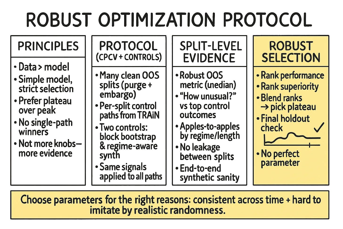
The answer is a unified protocol that embeds control-group testing inside combinatorial, purged cross-validation. It provides dozens of independent test sets by combining non-overlapping temporal folds while enforcing purging and embargo to block leakage. Within each test split, we then run the identical signal sequence against a swarm of realistic alternative return paths built from the training data only—via block bootstrap (to preserve local dependence and volatility clustering) and simple regime-aware synthetic generation (to probe beyond what the bootstrap can sample). The question is no longer “Did the strategy make money on this split?” but “How unusual was that PnL relative to what structured randomness typically produces on a path of this length and character?”

This yields two complementary pieces of evidence per parameter and per split: a robust performance summary and a conditional superiority probability—the fraction of top-decile control outcomes that the actual PnL beats. Aggregating across splits with medians (not means) gives each parameter a pair of stable, outlier-resistant scores: typical performance and typical superiority. Because these scores live on different scales, we move to a non-parametric decision space: rank each parameter on each metric, normalize ranks to [0,1], and blend them with a single weight that encodes your stance on performance versus robustness. The chosen parameter maximizes this composite rank; in practice it tends to sit on a flat plateau rather than a brittle peak.

Performance vs. Robustness

We live and die by our models. Yet, between a clever idea and a profitable strategy lies a treacherous minefield: parameter optimization. This initial dilemma is as old as the practice itself. Given a model structure, what parameters should we choose? The immediate, seductive answer is to pick the parameters that produced the best historical performance. But as we already know, this is optimization in its most naive form, and it's a well-trodden path to ruin.

Backtest optimization is an exercise in extreme order-statistic selection. We throw a grid of parameters at a finite dataset, and the optimizer, by its very nature, finds the one that perfectly exploited the quirks and idiosyncrasies of that specific historical path. It finds the winning lottery ticket from the past. The problem, of course, is that this perfection is brittle. The maximal Sharpe ratio or total PnL is often an outlier, a thin peak in the performance landscape forged by a confluence of serial dependence and random noise. The moment the market's character shifts, the strategy's edge, so finely honed to a past that will never repeat, shatters. The signal-to-noise ratio in financial data is notoriously low; naive optimization amplifies the noise and mistakes it for a signal.

This leads to the fundamental tension: we must optimize to specify our models, but the act of optimization itself is what makes them fragile. The quest, then, is not for the best parameter, but for the most robust one—a parameter whose effectiveness is not a statistical fluke. We can see this tension in the next image:

Along the horizontal axis sits model complexity; vertically, accuracy. The upper scale annotates robustness, which typically moves in the opposite direction of complexity: simpler models tend to be more stable under perturbations, while complex ones are more sensitive. On the left we have underfitting (high bias, low variance); on the right, overfitting (low bias, high variance). The central region is where bias and variance can be balanced—but only if we resist the temptation to push complexity to the rightmost edge.

The green curve (training accuracy) climbs and then plateaus—training error can always be reduced by adding complexity. The orange curve (test accuracy under an IID-like split) forms the familiar hump: performance improves with complexity up to a point and then degrades as variance dominates. The naive optimizer chases the orange peak, because that is where backtest metrics look their best.

The red curve is the crucial reality check: it represents performance when the test distribution is shifted or modified—exactly the market we trade in, where regimes, liquidity, and microstructure drift. Under shift, the peak moves down and to the left. In other words, the very complexity that squeezed out a few extra basis points in-sample is the first to break when the data-generating process wiggles. Robustness degrades fastest precisely where the backtest looked most impressive.

This is why the robustness/accuracy trade-off arrow in the diagram points to a point left of the test peak—at least in traditional parameter optimization . You intentionally give up a sliver of headline accuracy to land on a flatter summit—a parameter region whose neighborhood exhibits small performance gradients. Flatness here is not aesthetic; it is insurance. A broad plateau implies that modest shifts in market conditions, execution frictions, or sampling quirks do not produce large swings in realized PnL.

Said differently: the choice is not between best and second best, but between a narrow, high peak that is brittle and a lower, wide plateau that is resilient. The latter aligns with our objective: survive distribution shift and transaction realities while preserving edge. The diagram’s bias-variance annotations simply remind us that both extremes—too simple or too complex—are failures for different reasons; robustness lives in the middle, and a little to the left of whatever your pristine backtest crowned as “optimal.”

Now, in this article, we're going to develop a new protocol that combines two methods we've previously seen in other articles, but applied to other contexts. I recommend you read them before continuing, because many of the things we'll cover are continuations of the previous ones.

[WITH CODE] Combinatorial Purged Cross Validation for optimization

[WITH CODE] Evaluation: Validation framework

Risks and model limitations

A combined Combinatorial Purged Cross-Validation (CPCV) and Control-Group framework seems like a silver bullet. CPCV addresses the problem of temporal dependence and path dependency by creating numerous, independent out-of-sample test sets from the training data. It asks:

• Is the parameter's performance stable across different market periods?

• Control groups, on the other hand, tackle the problem of randomness.

They ask a different question: Is this performance, even if stable, statistically unusual when compared to realistic, random-but-structured alternatives?

However, bolting these two methods together is not straightforward. A naive implementation is fraught with risks that can undermine the entire validation process:

1. Purging and embargoing are essential in CPCV to prevent the training sets from "seeing" information from the test sets. An incorrect implementation leads to inflated and misleading performance estimates.

2. The power of a control group lies in its realism. A block bootstrap that uses the wrong block-length distribution or a synthetic data generator that fails to capture path volatility will create weak, unrealistic counterfactuals. If your random benchmarks are too easy to beat, the test is meaningless.

3. A critical, yet subtle, error is to use information from the test set path to construct the control groups for that same path. Control groups must be built only from the training data, preserving the out-of-sample integrity of the test.

4. How do you combine the scores from dozens of CPCV splits? Averaging performance metrics like Sharpe ratios across heterogeneous splits (e.g., a quiet period vs. a volatile crisis) can be misleading. A single outlier split can dominate the mean, masking the true typical performance.

5. In a parallelized environment, if different worker processes share the same random number generator state or accidentally share cached data, their trials are no longer independent. This can lead to correlated results that appear more significant than they are.

Parameter selection without a foundation

The core conflict is simple: the optimizer will always find something. It is a mathematical certainty. If you ask a machine to maximize a function over a grid, it will return a maximum. The pivotal event in a researcher's journey is the realization that this answer, by itself, is meaningless. The number it spits out lacks a foundation.

To build that foundation, we must subject any proposed parameter to two independent sources of evidence, answering two distinct questions:

1. Out-of-fold performance (CPCV): Does the parameter demonstrate stable, positive performance across multiple, distinct market environments, accounting for the temporal structure of the data? This removes leakage and reduces dependence on a single historical path.

2. Counterfactual superiority (Control groups): Is that performance genuinely exceptional, or could it be easily achieved by a random strategy operating under similarly realistic market conditions? This guards against selecting a parameter that was merely lucky.

A parameter is only chosen if it performs well in both dimensions. This dual-objective requirement is the foundation upon which a robust strategy is built. It is the core of the protocol we will now detail.

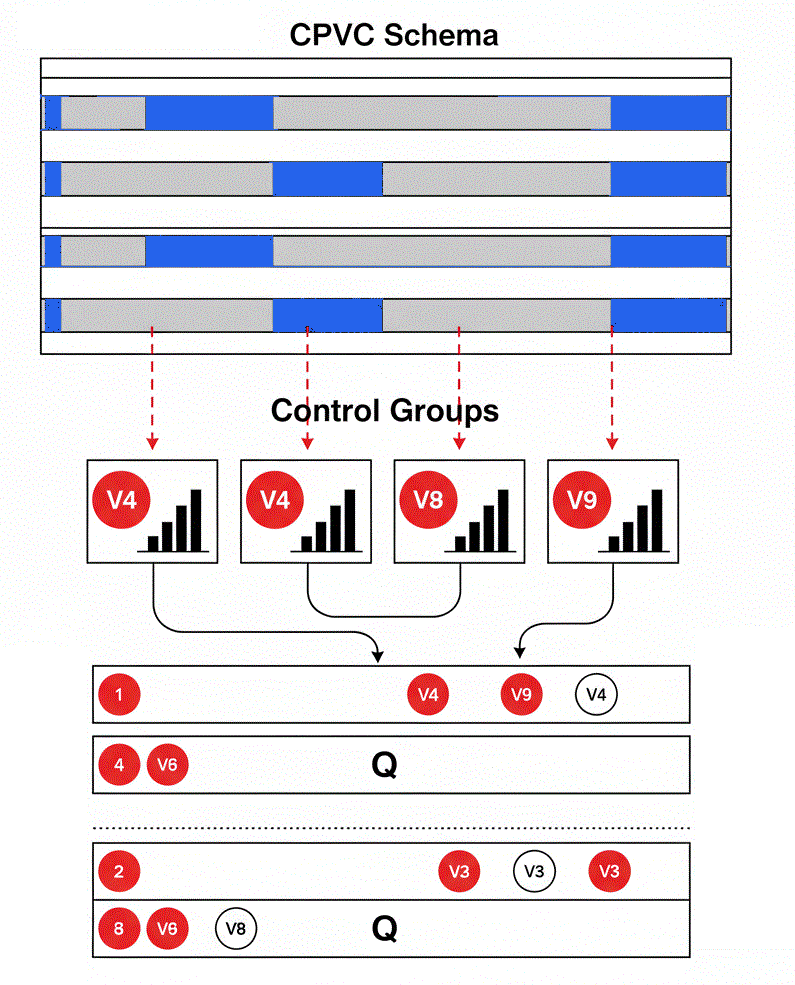
The central idea is to embed the control group test inside the CPCV loop. Instead of running one large cross-validation and then one large counterfactual test, we unify them. For each CPCV test split—each unique slice of market history—we don't just ask, How well did it do? We immediately follow up with a more critical question: How unusual was that performance for a path of this specific length and volatility character?

This per-split approach addresses the heterogeneity problem head-on. A strategy's performance in a low-volatility, trending market should be compared to random trials from that same regime, not to a generic baseline derived from all market types. By generating control groups calibrated to the training data but evaluated on each test split, we create a truly apples-to-apples comparison at every step.

This method transforms the output. Instead of just a distribution of Sharpe ratios from CPCV, we get a second, parallel distribution of probabilities—the probability that our strategy's performance on a given split was superior to a robust set of counterfactuals. The challenge then becomes selecting a parameter that is strong on both fronts: high, stable Sharpe and high, stable superiority.

To implement this vision, we must confront several technical and conceptual hurdles:

1. Both the validation (CPCV) and the resampling (Control groups) must be regime-aware. Financial markets are not stationary. Volatility, correlation, and drift change over time. Our entire framework must adapt to this reality, rather than assuming it away.

2. Purged and embargoed splits are non-negotiable. Control paths must preserve local dependence through block resampling or synthetic generation, not just draw from an i.i.d. pool.

3. The optimizer's curse is that it will maximize whatever metric it is given. If we just ask it to maximize the mean Sharpe, it will find a fragile peak. We need a more robust selection criterion. The solution is to rank and blend, moving from a parametric to a non-parametric selection space to avoid being fooled by the scale of the outputs.

4. A full CPCV is computationally expensive. Running thousands of control group paths for each CPCV split for each candidate parameter is prohibitively slow. The solution lies in aggressive caching (via length-keyed caches) and parallel evaluation.

5. Reproducibility: When randomness is a core part of the validation process (in resampling and split selection), ensuring that results are reproducible is paramount. This requires careful management of RNG seeds and isolation between parallel workers.

Robust optimization protocol

Here is where the technical details of the protocol are broken down into seven distinct stages that move from problem definition to final selection.

1. Problem statement and design goals:

Everything begins with a clear definition of the problem. We operate on two aligned time series:

• x_t: The driver series. This is the raw information source from which trading signals are generated. It could be a volatility index, a sentiment score, or any other feature.

• P_t: The price series. This is the instrument we trade. Its returns determine our profit and loss.

A model, parameterized by a set of hyperparameter, produces trading signals s_t(N)∈−1,0,1. These signals are generated exclusively from the driver series, x₁: t, to prevent any lookahead bias from the price itself.

The goal is to select the optimal parameter set, from the candidate space N.

The net returns of the strategy at time t are a function of the signal, the price change, and transaction costs. Assuming a latency of L periods between signal generation and execution, and a transaction cost c proportional to the size of the trade, the net return is:

\(r_t(N) = s_{t-L}(N)\Delta P_t - c \lvert s_{t-L}(N) - s_{t-L-1}(N) \rvert \quad \text{where} \quad \Delta P_t = P_t - P_{t-1}\)

This seemingly simple equation encodes our core objective. The entire validation framework is designed to find the optimal set of parameters that generates a sequence of returns r_t(N) that is not just profitable, but robustly so.

To achieve this, we impose a set of non-negotiable constraints on the design:

1. Split-level independence: The evaluation score for any given CPCV split must depend only on that split's test returns and the training data associated with it. No information can bleed across splits.

2. Training-only counterfactuals: The control paths used to test a split of length L must be derived only from the training returns. This is the cardinal rule to prevent double-dipping.

3. Robust aggregation: The final aggregation of scores across the numerous CPCV splits must be robust to outliers. This pushes us towards using medians instead of means.

We also operate under a key assumption known as local regime approximation:

While markets are globally non-stationary, we assume that within local windows, their statistical properties (like volatility) are stable enough to be modeled. The block bootstrap implicitly captures this, and our regime-aware synthetic data generation makes it explicit.

2. CV for dependent data:

Standard K-fold cross-validation is catastrophic for time-series data. It randomly slices up the data, shuffling the temporal order and leaking information from the future (training set) into the past (test set) through overlapping observations used in features or labels. Walk-forward validation is an improvement, but it's path-dependent and provides too few test sets.

Combinatorial Purged Cross-Validation is a possible solution as seen in previous articles. For each test splits, I, we generate the signals s_t(N) using the model and compute the net returns r_t(N) for t∈I. We then summarize the performance on this split using robust metrics. The most common is the Sharpe ratio:

\(\begin{align} \mathrm{Sharpe}_I(N) &= \frac{\bar r_I(N)}{\sigma_I(N) + \epsilon},\\[4pt] \text{where}\quad \bar r_I(N) &= \frac{1}{|I|}\sum_{t\in I} r_t(N),\\[4pt] \text{and}\quad \sigma_I(N) &= \sqrt{\frac{1}{|I|}\sum_{t\in I}\big(r_t(N)-\bar r_I(N)\big)^2 }. \end{align} \)

The small constant ϵ in the denominator prevents division by zero.

Here's a Python snippet that constructs the CPCV splits.

import numpy as np
import itertools
from typing import List, Optional

def _build_cpcv_splits(T: int, K: int = 10, m: int = 2, max_splits: Optional[int] = None) -> List[np.ndarray]:
    """
    Builds the indices for each CPCV test split.
    T: Total number of samples.
    K: Number of primary folds to partition the data into.
    m: Number of folds to combine for each test set.
    max_splits: If not None, randomly sample this many combinations.
    """
    if K < m:
        raise ValueError("K must be greater than or equal to m.")
    
    folds = np.array_split(np.arange(T, dtype=int), K)
    
    # Generate all possible combinations of m fold indices
    all_combos = list(itertools.combinations(range(K), m))
    
    # Subsample if requested
    if (max_splits is not None) and (max_splits < len(all_combos)):
        rng = np.random.default_rng(seed=2025) # Seed for reproducibility
        pick_indices = rng.choice(len(all_combos), size=max_splits, replace=False)
        all_combos = [all_combos[i] for i in pick_indices]
        
    test_splits = []
    for combo in all_combos:
        # Concatenate the folds corresponding to the current combination
        idx = np.concatenate([folds[i] for i in combo])
        test_splits.append(np.sort(idx))
        
    return test_splits

This function provides the core machinery for generating the diverse out-of-sample paths that form the first pillar of our validation.

3. Control-group testing on each split:

For each CPCV test split I, we have a vector of net returns r_I(N) and an actual, realized final PnL. Now we ask the crucial question: is this r_I(N) value special?

To answer this, we generate a large ensemble of realistic but random alternative price paths. These are our control groups. The key is that these paths are generated from the statistical properties of the training data only. We use two distinct but complementary methods to generate control returns, ensuring our conclusions are not an artifact of a single resampling technique.