

[WITH CODE] Evaluation: Validation framework
Third layer for multi‑testing strategy validation

Table of contents:
Introduction.
The Null Hypothesis framework in strategy validation.
Market state-conditioning.
The Timing Control Group Method.
The stationary Block Bootstrap.
The Stratified Synthetic data test.
Quantifying alpha with conditional superiority.
The multi-test validation framework.
Before you begin, remember that you have an index with the newsletter content organized by clicking on “Read full story” in this image.

Introduction
humanize it as if you were a senior quant: In the realm of quantitative finance, the allure of a pristine backtest—a smooth, upward-sloping equity curve—often masks a perilous truth: the line between genuine predictive skill and overfitting to historical noise is razor-thin.
Traditional performance metrics like the Sharpe ratio or total return, while informative, fail to answer the critical question: How likely is this performance to persist in unseen market conditions? This article introduces a rigorous framework for strategy validation that transcends naive backtesting, addressing the insidious risks of overfitting through a multi-dimensional statistical lens.
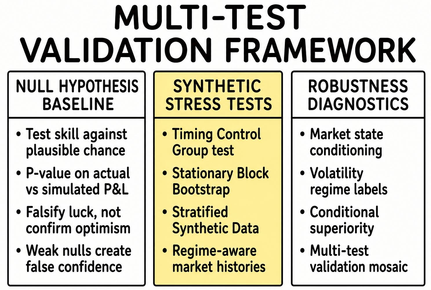
Building on prior discussions of backtesting methodologies, we shift focus from what a strategy achieved to why its performance matters. The core challenge lies in distinguishing strategies rooted in economic logic from those exploiting random patterns in historical data. To this end, we present a systematic approach anchored in three pillars:
Market regime conditioning: Acknowledging the non-stationary nature of financial markets by stratifying volatility regimes, ensuring robustness across changing dynamics.
Synthetic stress testing: Generating alternative market histories—via timing permutations, block-bootstrapped returns, and regime-driven synthetic data—to challenge a strategy’s adaptability.
Conditional superiority metrics: Moving beyond p-values to quantify a strategy’s ability to outperform even the top random outcomes from these tests, directly addressing its economic viability.
This framework does not seek to confirm a strategy’s profitability but to rigorously falsify the hypothesis that its success stems from luck. By isolating timing skill, path dependency, and regime-specific robustness, we provide a diagnostic toolkit to identify fragility before capital is deployed. As explored in earlier work, the stakes are high: deploying overfit strategies risks capital erosion, while dismissing skillful ones squanders opportunity. Here, we equip practitioners with the means to navigate this balance, transforming backtests from seductive illusions into credible evidence of alpha.
The first pillar , Market Regime Conditioning , confronts the non-stationary reality of financial markets. Historical returns are not independent, identically distributed (IID) events; instead, they cluster into distinct regimes characterized by volatility, trendiness, or mean reversion. By segmenting data into volatility quintiles, we create a stratified framework that tests whether a strategy’s success depends on specific market states or reflects broad adaptability. This approach prevents strategies from “hiding” in high-volatility environments where random trades may coincidentally profit, ensuring robustness across both tranquil and turbulent periods.
The second pillar, synthetic stress testing, introduces three complementary methodologies to stress-test a strategy’s resilience:
Timing Control Group (TCG) Test : Challenges the hypothesis that a strategy’s profitability stems from skillful trade timing rather than fortuitous market entry points. By reassigning trade initiation dates within the same volatility regime, we isolate timing luck and quantify whether the original strategy’s performance is statistically distinguishable from random permutations.
Stationary Block Bootstrap (BB) Test : Preserves temporal dependencies like autocorrelation and volatility clustering by resampling contiguous blocks of returns. This tests a strategy’s adaptability to alternative historical paths that retain the statistical DNA of real markets, exposing fragility to specific sequences of events.
Stratified Synthetic Data Test : Generates entirely new market histories using regime-specific distributions, blending real data with synthetic returns to simulate plausible yet unseen market dynamics. This pushes validation beyond historical repetition, probing whether a strategy captures structural truths rather than noise.
The third pillar , Conditional Superiority Metrics , elevates the analysis from rejecting randomness to quantifying economic significance. While p-values measure statistical significance, they do not address whether a strategy’s edge is practically meaningful. Conditional Superiority Probability (P_CS) answers this by asking: What is the likelihood that the strategy outperforms even the top random outcomes from these stress tests? For example, a P_CS(0.8) of 70% means the strategy beats 70% of the highest-performing random simulations, establishing a threshold for actionable alpha. This metric shifts the focus from avoiding Type I errors (false positives) to ensuring that surviving strategies deliver exceptional risk-adjusted returns.
The synthesis of these tests forms a Multi-Test Validation Framework , where no single result suffices. A strategy might pass the TCG test (indicating skillful timing) but fail the Block Bootstrap (revealing path dependency), or excel in synthetic data tests (proving regime-aware logic) yet stumble in timing permutations. By aggregating evidence across dimensions, we construct a mosaic of robustness that balances Type I and Type II errors: avoiding deployment of fragile strategies while preserving those with genuine skill masked by unlucky historical paths.
This framework is not a checklist but a scientific process of iterative falsification. Each test acts as an intellectual stress test, systematically dismantling the narrative of alpha until only strategies with structural integrity remain. The computational intensity of this approach is a necessary cost, dwarfed by the potential losses of deploying overfit models. Just as aerospace engineers simulate extreme turbulence to validate aircraft designs, quants must subject strategies to synthetic market histories that expose weaknesses invisible in traditional backtests.
The following sections detail the implementation of these tests, their interpretation, and their synthesis into a holistic validation process—a necessary evolution in an era where quantitative strategies must withstand not just the past, but the uncertainty of the future. By transforming backtests from seductive curves into evidence-based narratives, we empower practitioners to navigate the razor-thin line between insight and illusion with rigor, precision, and humility.
The Null Hypothesis framework in strategy validation
Before we can validate a strategy, we must first define what we are testing against. The common objective—to see if the strategy makes money—is statistically naive. A more rigorous question is: Does the strategy's performance significantly exceed what could be expected from a plausible null hypothesis?
The null hypothesis, H_0, posits that the observed profits are the result of chance, given the strategy's structural characteristics. Our task is to quantify the evidence against this hypothesis.
The primary tool for this is the p-value. In this context, the p-value represents the probability of observing a performance metric—final Profit and Loss—at least as extreme as the one achieved by the actual strategy, assuming the null hypothesis is true. A low p-value—typically < 0.05 or < 0.10—suggests that the observed performance is unlikely to be a random fluke, allowing us to reject the null hypothesis in favor of the alternative, which is that the strategy possesses genuine predictive skill.
We already went deeper in this article:

The calculation itself is straightforward. We generate a large number, N, of synthetic performance histories under a specific null hypothesis. Let the terminal P&L of the actual strategy be Pactual and the set of terminal P&Ls from the N simulations be P1, P2, ..., PN. The one-sided p-value is then calculated as:
where II(⋅) is the indicator function. The term for equality handles ties by distributing their probability mass, providing a more precise estimate.
In our framework, this is implemented with a simple, reusable function that takes the array of simulated profit paths and the actual final profit.
def _calculate_pvalue(self, paths: np.ndarray, actual_pnl_end: float) -> float:
    """
    Calculates the p-value for the actual performance against simulated paths.

    Args:
        paths: An (N, T) array where N is the number of simulations and T is time.
        actual_pnl_end: The final cumulative profit of the actual strategy.

    Returns:
        The p-value.
    """
    if paths.shape[0] == 0:
        return 1.0 # If no paths were generated, we cannot reject the null.

    # Count how many simulated paths ended with a higher P&L.
    greater = np.sum(paths[:, -1] > actual_pnl_end)

    # Count how many simulated paths ended with the exact same P&L.
    equal = np.sum(paths[:, -1] == actual_pnl_end)

    # Apply the formula.
    return (greater + 0.5 * equal) / len(paths)
The crucial part of this framework is not the calculation itself, but the generation of the synthetic paths. The definition of the null hypothesis dictates how these paths are created. A poorly chosen null hypothesis can lead to misleading p-values.
For instance, assuming returns are independent and identically distributed is a weak null hypothesis, as it ignores known market phenomena like volatility clustering and autocorrelation. The remainder of this article is dedicated to constructing and implementing more realistic and challenging null hypotheses to rigorously test our strategies.

Market state-conditioning
Financial market returns are not stationary; their statistical properties change over time. One of the most prominent features of market data is volatility clustering, where periods of high volatility are followed by more high volatility, and tranquil periods are followed by more tranquility. A sophisticated trading strategy should, implicitly or explicitly, adapt to these changing conditions. Consequently, a robust validation framework must account for them.
We introduce the concept of market regimes, defined here by the prevailing level of market volatility. By stratifying the time series into distinct volatility regimes, we can construct more plausible null hypotheses. For example, a test can be designed to assess whether a trade's profitability was due to skill or merely due to it being placed in a high-volatility environment where large price swings are common.
The first step is to compute a rolling measure of volatility. We use the rolling standard deviation of returns. A numerically stable and efficient method to compute this utilizes convolution.
Rolling volatility calculation
The sample standard deviation over a window of size w is
This can be rewritten in terms of means of powers:
We can compute the rolling mean E[X] and the rolling mean of squares E[X2] efficiently using np.convolve.
def _rolling_std(self, arr: np.ndarray, window: int) -> np.ndarray:
    """
    Calculates the rolling standard deviation using convolution for efficiency.
    This applies Bessel's correction (ddof=1).
    """
    if window < 2:
        return np.zeros_like(arr)

    # A flat kernel to compute the moving average.
    kernel = np.ones(window) / window

    # Compute the rolling mean of the array and the array of squares.
    mean = np.convolve(arr, kernel, mode='valid')
    mean_sq = np.convolve(arr**2, kernel, mode='valid')

    # Calculate the sample variance. The term (window / (window - 1)) is Bessel's correction.
    var = (mean_sq - mean**2) * (window / (window - 1))

    # Ensure variance is non-negative due to potential floating point errors.
    std = np.sqrt(np.maximum(var, 0))

    # Pad the result to match the original array's length.
    result = np.zeros_like(arr)
    result[window - 1:] = std
    return result
Regime labeling
Once we have the time series of rolling volatility, we can partition it into quantiles to define our regimes. For example, we can define 5 regimes where Regime 0 is the lowest volatility quintile, and Regime 4 is the highest.
def _label_regimes(self):
    """
    Labels each time point with a volatility regime.
    """
    window = 20 # The lookback window for volatility calculation.
    vol = self._rolling_std(self.returns, window)

    # We can only define thresholds based on the valid, non-zero volatility values.
    valid_vol = vol[window:]
    if valid_vol.size > 0:
        # Define the quantile boundaries for n_regimes.
        # e.g., for 5 regimes, we need the 20th, 40th, 60th, 80th percentiles.
        thresholds = np.percentile(
            valid_vol, np.linspace(0, 100, self.n_regimes + 1)[1:-1]
        )
    else:
        thresholds = [] # Not enough data.

    # Label each time step based on which threshold its volatility surpasses.
    self.regimes = np.zeros(self.T, dtype=int)
    for r, th in enumerate(thresholds, start=1):
        self.regimes[vol >= th] = r
The output of this process is an array, self.regimes, of the same length as our price series, where each element is an integer label for the market state at that time. This state-conditioning is a foundational component for the advanced tests that follow.
The visualization below shows a sample price series with the background colored according to the calculated volatility regime. This clearly illustrates how market dynamics are segmented.
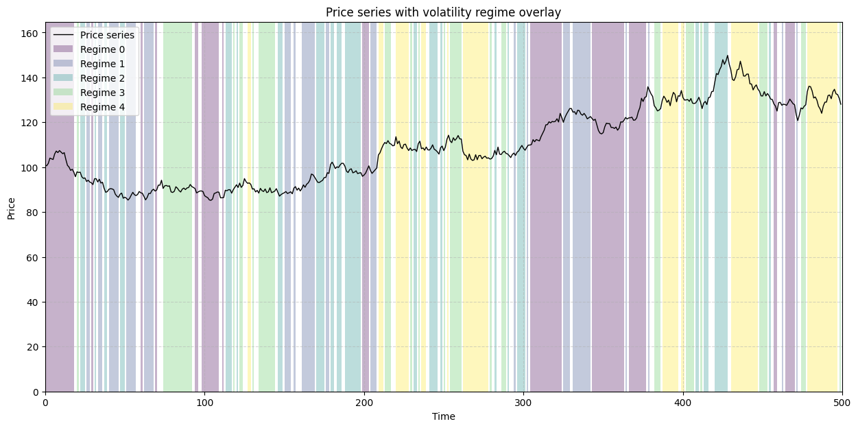
This explicit acknowledgment of changing market states allows us to build null hypotheses that are far more credible and challenging to overcome than simple random shuffles.
The Timing Control Group method
The first advanced test we introduce directly addresses the problem of timing luck. A strategy might generate profits not because its signals are inherently predictive, but because they happened to occur at fortuitous moments. The Timing Control Group (TCG) test evaluates this by asking: Given the set of trades the strategy identified, what would the performance have been if those trades had been initiated at other, plausible times?
The null hypothesis for the TCG test is: The profitability of the strategy is not dependent on the specific timing of its trades, only on the market regimes in which they were placed.
The procedure is as follows:
Deconstruct the signal: First, we parse the raw signal vector (e.g.,
[0, 1, 1, 1, 0, -1, -1, 0]) into a list of discrete trading segments. Each segment contains its start time, duration, direction (long/short), and, critically, the volatility regime that was active at its inception.Create a pool of alternatives: For each actual trade segment, we create a pool of all possible alternative start times. An alternative is considered valid only if it occurs within the same volatility regime as the original trade and allows for the full duration of the trade to complete.
Generate synthetic histories: We construct N synthetic signal vectors. Each synthetic history is built by taking every trade from the original strategy and randomly re-assigning its start time to one of the valid alternatives from its pool.
Calculate P&L and p-value: We compute the P&L for each of the N synthetic histories and use this distribution to calculate a p-value for the actual strategy's performance.
This method preserves the exact number, duration, and regime-context of the trades, isolating the impact of timing alone. The implementation begins by extracting the trade segments.
def _extract_segments(self, sig: np.ndarray):
    """
    Parses a signal vector into a list of trade segments.
    Each segment is a tuple of (start, duration, sign, regime).
    """
    segments = []
    t = 0
    while t < self.T:
        if sig[t] != 0:
            sign = sig[t]
            start = t
            t += 1
            while t < self.T and sig[t] == sign:
                t += 1
            dur = t - start
            reg = self.regimes[start] # Regime at the start of the trade
            segments.append((start, dur, sign, reg))
        else:
            t += 1
    return np.array(segments, dtype=int)
Next, the main function generates the synthetic paths by sampling from the regime-conditioned pools.
def timing_controlgroup(self, N=1000, seed=None):
    """
    Runs the Timing Control Group test.
    """
    rng = np.random.default_rng(seed)
    self.pvalues_timing = np.zeros(self.n_strats)
    self.controlgroup_paths_timing = []

    for i in range(self.n_strats):
        segs = self._extract_segments(self.signals[i])
        paths = np.zeros((N, self.T))

        if segs.size:
            for j in range(N):
                exp = np.zeros(self.T) # Synthetic exposure vector
                # For each actual trade...
                for _, dur, sign, reg in segs:
                    # Find all valid start times in the same regime.
                    valid_starts = np.where(self.regimes[:self.T - dur] == reg)[0]
                    if len(valid_starts) > 0:
                        # ...and randomly pick one to initiate the trade.
                        s = rng.choice(valid_starts)
                        exp[s:s + dur] += sign

                # Calculate the P&L for this synthetic path.
                paths[j] = np.cumsum(exp * self.returns)

        self.controlgroup_paths_timing.append(paths)
        actual_end = np.cumsum(self.signals[i] * self.returns)[-1]
        self.pvalues_timing[i] = self._calculate_pvalue(paths, actual_end)
A low p-value from the TCG test provides strong evidence that the strategy's timing is skillful. Conversely, a high p-value (e.g., > 0.2) is a significant warning sign, suggesting that the historical performance was heavily reliant on lucky timing that is unlikely to be replicated.
The visualization below shows the actual P&L curve against the confidence band of P&L from the thousands of randomly-timed synthetic histories.
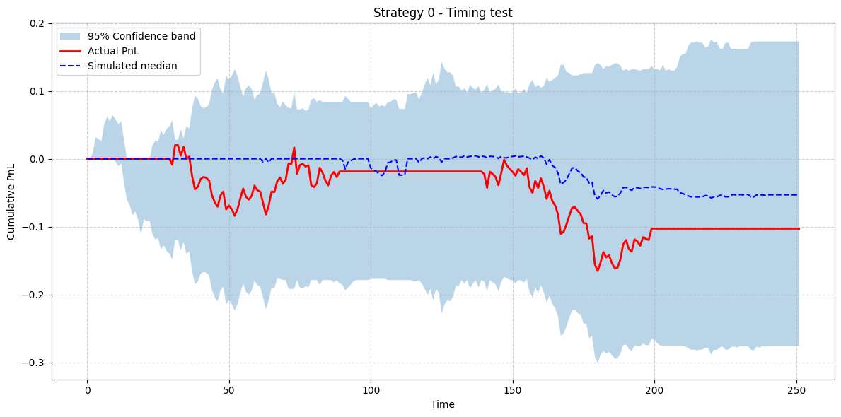
If the red Actual PnL line resides comfortably above the blue cloud of randomness, it indicates that the strategy's timing was consistently better than random selections within similar market conditions.
The stationary Block Bootstrap
The TCG test is excellent for analyzing timing luck but operates on a fixed history of returns. It doesn't answer the question: How would this strategy have performed on a different, but statistically similar, historical path?
To address this, we need to resample the returns themselves. A naive shuffle of daily returns would destroy crucial temporal structures like autocorrelation and volatility clustering.
The Stationary Block Bootstrap (BB) is a resampling technique designed to preserve these dependencies. Instead of resampling individual returns, it resamples blocks of contiguous returns. By keeping these blocks intact, we retain much of the short-term autocorrelation structure of the original series.
The null hypothesis for the BB test is:
The strategy's performance is not due to skill but is an artifact of applying its fixed rules to a specific historical return series. It would not be profitable on other series with similar short-term statistical properties.
The procedure is as follows:
Define block sampling: Blocks of returns are drawn with replacement from the original series. To avoid artifacts from using a fixed block size, the length of each block, L, is drawn from a probability distribution. We use a Geometric distribution, as it's memoryless and simple to implement. The mean block size is a key parameter.
Construct bootstrapped return series: We create N new return series, each of length T. Each series is constructed by repeatedly drawing blocks of returns and concatenating them until the desired length is reached.
Apply fixed signal: The original, unchanged signal vector is applied to each of the N bootstrapped return series to generate N synthetic P&L paths.
Calculate p-value: The distribution of terminal P&Ls from these paths is used to compute a p-value for the strategy's actual performance.
The core of the implementation is the loop that generates the bootstrapped return series.
def block_bootstrap(self, N=1000, seed=None):
    """
    Runs the Stationary Block Bootstrap test.
    """
    rng = np.random.default_rng(seed)
    self.pvalues_block = np.zeros(self.n_strats)
    self.bootstrap_paths = []

    # The parameter for the geometric distribution.
    # The mean block length will be self.block_min.
    p_geom = 1.0 / self.block_min

    for i in range(self.n_strats):
        sig = self.signals[i]
        paths = np.zeros((N, self.T))

        for j in range(N):
            boot_returns = []
            while len(boot_returns) < self.T:
                # Draw block length from a clipped geometric distribution.
                blen = np.clip(rng.geometric(p_geom), self.block_min, self.block_max)

                # Randomly choose a starting point for the block.
                start = rng.integers(0, self.T - blen + 1)

                # Append the block of returns.
                boot_returns.extend(self.returns[start:start + blen])

            # Apply the original signal to the new return series.
            paths[j] = np.cumsum(sig * np.array(boot_returns[:self.T]))

        self.bootstrap_paths.append(paths)
        actual_end = np.cumsum(sig * self.returns)[-1]
        self.pvalues_block[i] = self._calculate_pvalue(paths, actual_end)
The use of np.clip with rng.geometric ensures that the blocks are of a reasonable size, preventing the selection of overly short or long blocks that could distort the test.
The BB test assesses the strategy's robustness to variations in the market's path. A low p-value suggests the strategy is not just fit to one specific sequence of events but can likely handle different arrangements of historical market dynamics. A high p-value indicates the strategy's success might be fragile and highly dependent on the particular sequence of returns observed in the backtest period.
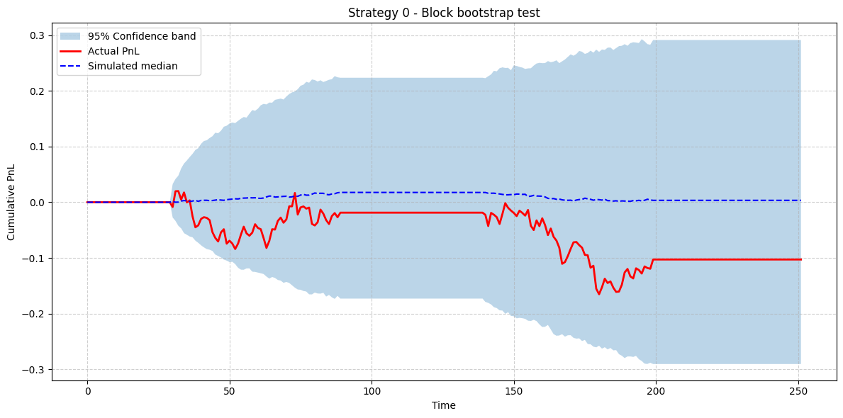
As before, the actual P&L (red) should ideally be above the confidence band of the bootstrapped results (blue). This test complements the TCG by stressing the strategy against a different dimension of randomness: the path of the market itself.

The Stratified Synthetic Data test
While the Block Bootstrap resamples from history, the Stratified Synthetic Data test goes a step further: it generates entirely new, artificial return series based on the statistical properties of the observed market regimes. This is the most interesting test in our framework, as it creates market scenarios that have never happened but are statistically plausible according to the regime model.
The procedure is as follows:
Characterize regimes: For each volatility regime r identified in Section 2, compute the sample mean and standard deviation of the returns in that regime:
Generate synthetic returns: At each time t, draw a synthetic return from the Normal distribution corresponding to its regime:
\(R_{\mathrm{synth},t}\;\sim\;\mathcal{N}\!\bigl(\mu_{\mathrm{regime}(t)},\,\sigma_{\mathrm{regime}(t)}\bigr).\)Blend with real data: Combine the actual return Ractual,t and the synthetic return Rsynth,t via
\(R_{\mathrm{final},t} = \alpha\,R_{\mathrm{actual},t} + (1 - \alpha)\,R_{\mathrm{synth},t}.\)The correlation factor α∈[0,1] tunes the test’s difficulty:
A high (e.g. 0.9) yields paths very close to the historical series.
A low (e.g. 0.2) produces more randomized trajectories, while preserving the regime structure.
Apply signal and test: Apply your original trading signal to each of the N blended return series {Ractual,t}. From the resulting P&L paths you then compute the final p-value.
The code first computes the statistics for each regime and then generates the blended synthetic series in a loop.