[WITH CODE] Combinatorial Purged Cross Validation for optimization
Parameter optimization part II
Table of contents:
Introduccion.
Is robustness pure fiction?
Risks and limitations of this approach.
Model specification and parameter dependency.
The illusion of optimal.
The failure of standard CV in finance.
Probabilistic framework.
The Probabilistic Sharpe Ratio and robustness metrics.
A weighted consensus for stability.
Introduccion
Traditional grid or Bayesian searches conducted on a single path reward parameters that overfit to this specific historical path. This inflates performance metrics through selection bias and temporal leakage. Combinatorial Purged Cross-Validation (CPCV) addresses this flaw by generating a multitude of chronology-respecting train-test partitions. Crucially, it purges any overlapping information, ensuring that each out-of-sample evaluation is statistically independent of its training window.
The outcome is not a single performance score per parameter set, but rather an empirical distribution of out-of-sample outcomes. This distribution reveals the stabilityβor lack thereofβof the strategy across a diverse set of plausible historical paths. Consequently, the objective shifts from maximizing a point estimate to identifying robust parameter regions. We seek plateaus, not peaks: parameters that remain performant under numerous counterfactual scenarios are preferred over those that are optimal in one specific history but brittle elsewhere.
This conceptual reframingβfrom optimization to robustnessβestablishes the foundational framework for the subsequent analysis. In fact, today we're going to look at a different application than the classic use of CPCV.
Although the application context we'll be using has changed, you can find the classic uses here::
Ok, letβs continue! A common approach to this problem is to test a range of parameter values against historical data and select the combination that yields the highest performance. While intuitively appealing, this process is fraught with peril. The primary risk is selection bias, a specific and insidious form of overfitting. By selecting the best-performing parameter set from a multitude of trials on the same historical data, we are often just fitting the model to the specific noise and random fluctuations of that particular history. The chosen optimal parameter is unlikely to be truly optimal for future, unseen data. It is merely the parameter that best memorized the past.
The danger of using a technique like CPCV without a deep understanding of its purpose is that it can be misconstrued as just another, more complex, way of finding the peak of a profit-and-loss curve. One might run thousands of combinatorial paths, find the parameter value that appears most frequently among the top performers, and declare victory. This, however, is a subtle but critical failure. We are not looking for the best performance, but the most stable performance. The risk is overfitting the validation process itself, finding a parameter that looks robust by sheer chance across a specific set of random data splits.
Consequently, a single optimal parameter derived from a single historical path is a statistical illusion. The conflict is between our innate desire for a single, definitive, correct answer and the stark reality of a stochastic world where no such answer exists. This requires a fundamental shift in perspective: from optimization to robustness. The goal is not to find the parameter that would have been the best, but to find a parameter that is likely to be good enough across a wide range of plausible future scenarios. This shift is the intellectual engine driving the adoption of sophisticated validation techniques like CPCV.
Is robustness pure fiction?
If you have created a model, it is normal to have at least one parameter. And this is where the first problem comes in: The necessity of finding robust parameters is a prerequisite for survival in financial markets.
A strategy whose performance is highly sensitive to small changes in its parameters is inherently fragile. If a strategy is profitable with a 20-day lookback but incurs losses with a 19-day or 21-day lookback, its observed profitability was likely a statistical artifact, a result of overfitting to a specific frequency in the historical noise spectrum. The market does not operate on integer-day cycles with knife-edge precision. A truly robust strategy, one that has captured a genuine economic or behavioral anomaly, should exhibit a degree of performance stability across a neighborhood of similar parameter values.
This meta-stability is what provides confidence that the strategy's logic is sound. Therefore, the search for optimal parameters is not merely about maximizing a backtested performance metric; it is a search for evidence that our model is not a fluke.
The obstacles to achieving this are significant and scale poorly. Even when optimizing a single parameter, the primary challenge is the trade-off between bias and variance. If we use too little data for training (high bias), the model won't capture the underlying signal. If we use too much data and test too many parameter variations (high variance), we risk fitting to noise. This problem is amplified exponentially when we consider multiple parametersβa phenomenon known as the curse of dimensionality.
Consider a strategy with just three parameters, each with ten possible values. The total number of combinations to test is 103=1000. With five such parameters, it explodes to 105=100,000. The computational burden becomes immense, but more critically, the probability of finding a seemingly brilliant result purely by chance (a "false positive") approaches certainty. For a sufficiently large search space, the maximum of a set of random variables will almost always appear impressively high. This is why any of us need a statistically sound validation framework, to protect us from our own data-mining capabilities.
Risks and limitations of this approach
The logic of CPCV is significantly more complex than a standard backtest. Implementing the purged splitting, managing the combinatorial paths, calculating performance distributions, and aggregating results requires careful coding. This complexity creates a high risk of bugs that are not immediately obvious. For example:
An off-by-one error in the purging logic could re-introduce data leakage in a subtle way.
Incorrectly handling the indices for train/test splits could lead to lookahead bias.
Bugs in the calculation of higher-moment statistics (skew, kurtosis) could invalidate the PSR results.
The most dangerous aspect is that these bugs often result in silent failures: the code runs without crashing and produces a result, but that result is fundamentally flawed, leading to a false sense of confidence in a parameter or strategy.
Perhaps this is not the worst; there are more dramatic blunders, such as statistical or methodological ones. These risks are more subtle and relate to the statistical assumptions and limitations of the method itself.
CPCV is designed to prevent overfitting a parameter to a single historical path. However, if a researcher tests dozens of different strategy ideas (different models, different indicators, different rules) on the same dataset, all using a rigorous CPCV process, they will eventually, by pure chance, find an idea that looks robust. This is overfitting the research process or meta-overfitting. The researcher is selecting the luckiest outcome not from a set of parameters, but from a set of strategies. CPCV cannot protect you from this. The only defense is a disciplined research process, a strong economic rationale for each strategy, and the use of a final, untouched hold-out dataset.
The CPCV process itself has several key hyperparameters, and the final robust parameter can be sensitive to their settings:
n_splits
: The number of combinatorial paths. If this is too low (e.g., < 100), the resulting performance distributions will be unstable and noisy. The 10th percentile metric will not be reliable.train_size_pct
/test_size_pct
: This defines the bias-variance trade-off of the validation itself. Very short test sets will produce noisy performance metrics (high variance). Very short training sets will lead to poorly fitted models in each fold (high bias), underestimating the strategy's true potential.purge_size
: This is not a parameter to be guessed. It must be set based on the maximum horizon of your signal's dependency on future data. Setting it too small will fail to prevent leakage.
CPCV's core strength is testing a parameter against a wide combination of past market regimes. However, it operates on the fundamental assumption that the future will be a recombination of the past. It cannot anticipate a true structural break or a novel market regime with dynamics completely unseen in the historical data (e.g., a shift from inflationary to deflationary macro environments, or the introduction of a game-changing technology). A parameter found to be robust on 2000-2025 data is not guaranteed to be robust in a future regime that is fundamentally different from anything in that period.
CPCV requires a sufficiently long time series to be effective. If you are working with an asset that has limited history (e.g., a recently launched ETF or a cryptocurrency), CPCV is often impractical. The train and test windows would be so short that any performance metric calculated on them would be statistically meaningless. Attempting to use CPCV on insufficient data will produce unstable and unreliable results.
Besides we need to take into account the risks related to how the researcher interprets the output of the CPCV process, potentially leading to flawed conclusions.
The complexity and computational intensity of CPCV can create a powerful illusion of objectivity. Because the process is so involved and data-driven, it's easy to blindly trust the number it produces. A researcher might find that N=31 is the robust parameter and stop thinking, ignoring the fact that the underlying economic thesis for the strategy makes no sense at that frequency. The quantitative output must always be subject to qualitative oversight and economic reasoning.
The framework detailed in the paper focuses on the 10th percentile of the PSR distribution. This is an excellent metric for a strategy that aims for consistent, steady returns. However, it may be the wrong metric for other types of strategies. For example:
Crisis alpha / tail hedging strategy: Such a strategy is designed to lose small amounts of money most of the time and make very large gains during market crashes. Optimizing for the 10th percentile PSR would likely discard such a strategy. For this, one should analyze the 1st or 5th percentile of the returns distribution, not the PSRβthat we will be using for the sake of the article.
High-risk, high-reward strategy: For a strategy where the goal is to maximize upside, focusing on the 90th percentile of the distribution might be more appropriate. The key risk is misaligning the statistical metric used for optimization with the stated economic objective of the trading strategy.
Model specification and parameter dependency
To explore the nuances of parameter optimization, we must first define a model to operate on. For this exercise, we'll use a simple, yet effective, breakout strategy. The logic is straightforward: a signal is generated when the current price exceeds the maximum (for an upside breakout) or falls below the minimum (for a downside breakout) of a preceding number of periods. This number of periods is our key parameter, which we'll call the lookback window, denoted as N.
Mathematically, for a given price series P={p1,p2,...,pt}, the conditions for generating a signal at time t are:
Upside breakout signal (sell): ptβ>Htβ(N)
Downside breakout signal (buy): pt<Ltβ(N)
This model, while simple, encapsulates the fundamental challenge. The performance of the strategy is entirely dependent on the choice of N. A small N will make the model highly sensitive and prone to generating many signals, potentially capturing short-term moves but also getting whipsawed by noise. A large N will make the model less sensitive, generating fewer signals that correspond to more significant, sustained trends, but it might miss shorter-term opportunities and react slowly to market changes.
Let's implement this in Python.
import numpy as np
class BreakoutModel:
"""
A generic model to detect breakouts in a price series using NumPy.
An 'up' direction breakout occurs when the current price exceeds the max of the previous N bars.
A 'down' direction breakout occurs when the current price falls below the min of the previous N bars.
"""
def __init__(self, window: int = 20, direction: str = 'up'):
"""
Initializes the breakout model.
:param window: The lookback window (N) for calculating the max/min.
:param direction: 'up' for upside breakouts, 'down' for downside breakouts.
"""
if not isinstance(window, int) or window <= 0:
raise ValueError("window must be a positive integer.")
if direction not in ('up', 'down'):
raise ValueError("direction must be 'up' or 'down'")
self.window = window
self.direction = direction
def predict(self, data: np.ndarray) -> np.ndarray:
"""
Generates trading signals based on the breakout logic.
:param data: A NumPy array of prices.
:return: A NumPy array of signals (1 for buy, -1 for sell, 0 for no signal).
"""
data = np.asarray(data, dtype=float)
n_samples = len(data)
signals = np.zeros(n_samples, dtype=int)
# We can only start generating signals after the first full window
for i in range(self.window, n_samples):
window_slice = data[i - self.window : i]
if self.direction == 'up':
# An upside breakout is a signal to sell (e.g., shorting volatility)
if data[i] > np.max(window_slice):
signals[i] = -1
else: # direction == 'down'
# A downside breakout is a signal to buy (e.g., going long volatility)
if data[i] < np.min(window_slice):
signals[i] = 1
return signals
The code directly translates our mathematical definition. It iterates through the variable with predictive power and, for each point after the initial window, checks for the breakout condition.
The illusion of optimal
The most common and catastrophic mistake in parameter selection is naive in-sample optimization, a practice more accurately described as curve-fitting. This involves running a backtest for every possible parameter value in a given range on the entire historical dataset and selecting the value that produces the best result. The outcome is a parameter that is perfectly tailored to the specific quirks and random noise of that historical data, and almost certainly suboptimal for the future.
The probability of backtest overfitting is not just a qualitative concern; it can be quantified. Let N be the number of independent trials (e.g., the number of different parameter sets tested). If each trial's performance is a random variable, the expected value of the maximum performance across all trials will be significantly higher than the expected value of any single trial. This difference grows with N. By selecting the maximum, we are systematically selecting for positive estimation error. A metric like the Deflated Sharpe Ratio attempts to correct for this by estimating what the Sharpe Ratio would be if the selection bias were removed. Its calculation involves the variance of the tested Sharpe Ratios and the size of the trial set, effectively penalizing strategies that arise from extensive data mining.
Let's demonstrate this overfitting trap visually. We will split a historical price series into two parts: an in-sample (IS) set (e.g., the first 70% of the data) and an out-of-sample (OOS) set (the remaining 30%). We will perform a naive optimization on the IS set to find the best parameter N, and then we will observe the performance of all tested N values on the OOS set.
We will need these helpers:
def backtesting(price: np.ndarray, signals: np.ndarray) -> np.ndarray:
price_diff = np.diff(price, prepend=price[0])
signals_shifted = np.roll(signals, 1)
signals_shifted[0] = 0
strategy_returns = signals_shifted * price_diff
return np.cumsum(strategy_returns)
def model_signal_generator(series: np.ndarray, N: int) -> np.ndarray:
model_buy = BreakoutModel(window=N, direction='down')
model_sell = BreakoutModel(window=N, direction='up')
signals = model_buy.predict(series) + model_sell.predict(series)
position = 0
final_signals = np.zeros_like(signals)
for i in range(len(signals)):
if signals[i] != 0:
position = signals[i]
final_signals[i] = position
return final_signals
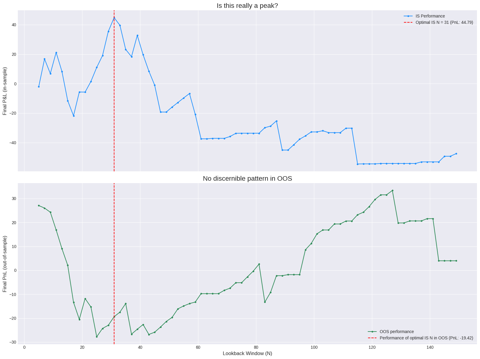
The visual evidence is damning. The top plot shows a classic, seductive optimization curve with a clear peak. An unsuspecting analyst would confidently select N=31. The bottom plot reveals the truth. The out-of-sample performance curve is a noisy, random-looking series with no discernible peak. The parameter that was optimal in-sample is unremarkable out-of-sample; its performance is mediocre, close to the average. This experiment starkly illustrates that the peak found in-sample was an artifact of fitting to noise. Maximizing performance on a single pass of the data tells us nothing about a parameter's robustness; in fact, it often leads us to select the least robust, most overfit candidates.
The failure of standard CV in finance
The obvious next step to mitigate overfitting is cross-validation (CV). The standard technique in mainstream machine learning, k-fold CV, involves splitting the dataset into k equal-sized folds. The model is then trained on kβ1 folds and tested on the remaining fold. This process is repeated k times, with each fold serving as the test set once. The performance is then averaged across all k trials. This process is designed to give a more reliable estimate of model performance on unseen data by using all the data for both training and testing at different stages.
While this is a cornerstone of validation in many domains, standard k-fold CV is fundamentally invalid for financial time series. Applying it correctly requires that the data points are independent and identically distributed. Financial data violates this assumption spectacularly. This failure stems from two critical properties:
Autocorrelation: The value of the series at time t is not independent of its value at tβ1. This serial dependence is the very phenomenon most trading strategies seek to exploit. Shuffling the data before performing k-fold CV, a common practice to ensure random folds, would completely destroy the temporal structure that gives the data meaning, rendering the validation exercise useless.
Data leakage/lookahead bias: This is a more subtle but equally fatal flaw. Even if we don't shuffle the data and create sequential folds, the standard k-fold structure allows future information to contaminate the training set. For example, a 5-fold split on 10 years of data might use years 1-2, 3-4, 7-8, and 9-10 for training, and test on years 5-6. The model being tested on 2015-2016 data would have been trained on data from 2017-2020. It has seen the future. This lookahead bias leads to wildly inflated and unrealistic performance estimates.
A better, though still imperfect, approach is Walk-Forward. In this method, the data is split into sequential chunks. The model is trained on chunk 1 and tested on chunk 2, then trained on chunks 1-2 and tested on chunk 3, and so on. This expanding window approach always respects the arrow of time. However, it is highly path-dependent. The resulting optimal parameter is tailored to the specific historical sequence of market regimes. If the last few folds of the data were a strong bull market, the process will favor parameters suited for that environment, which may not be robust overall. It also provides only a small number of test sets, making the final performance average potentially unstable. A more flexible and robust method is required.
To properly find the parameters we are looking for, we must construct our train/test splits in a way that prevents any form of informational leakage from the future to the past. Marcos Lopez de Prado, in his seminal work proposed a solution that addresses the data leakage problem, which is especially pernicious when labels themselves are forward-looking. This involves two key concepts: purging and embargoing.
The core principles of purging and embargoing remain identical to the machine learning context, but their role and application shift slightly when we move from fitting a classifier to optimizing a strategy's parameters. The fundamental goal is the same: to ensure the statistical integrity of the validation process by preventing information from the future (the test set) from contaminating decisions made in the past (the training set).
Let's translate the concepts:
In ML classification algos: The training process is about fitting a model (e.g., a random forest) to data to learn a pattern. The risk is the model learning from labels that were derived using test set information.
In CPCV parameter optimization: The training process isn't about fitting a model in the same way. Instead, for each of the hundreds of CPCV splits, the training phase consists of evaluating a range of different parameter values (e.g., N=10, 20, 30...) on the training portion of the data to find which parameter performs best within that specific training segment.
In the optimization context, purging ensures that the performance evaluation of different parameters on the training set is not tainted by the upcoming test set.
Imagine one of the random splits generated by CPCV:
Training Set: Indices 100 to 800
Test Set: Indices 820 to 1000
The training step involves a sub-competition: we test various parameter values (e.g., N
=10, 11, 12...) on the data from index 100 to 800. We might rank them by their Sharpe Ratio or another metric calculated only on this training slice.
The problem arises if the strategy logic or the metric used for this evaluation is forward-looking. For example, even if the trading signals themselves aren't forward-looking, a common practice is to use meta-labels or filters. A researcher might add a rule that a signal is only valid if the market's volatility in the next 3 days remains low.
How leakage occurs: If we evaluate a parameter's performance at index 798 of the training set, a 3-day forward-looking rule would depend on data at indices 799, 800, and 801. However, the true prices that will be used in the test set (starting at 820) are supposed to be unknown. Allowing any information, however indirect, about the test period to influence the selection of the best parameter during the training stage constitutes leakage.
The purging solution: The purge creates an informational air gap. It discards the end portion of the training set (e.g., indices 790-800) from the parameter-selection competition. This guarantees that no matter which parameter is being evaluated on the training data, its performance is judged on a set of data that is cleanly and completely separated from any information related to the upcoming test set.
On the other hand, embargoing ensures that each of the hundreds of test paths is as statistically independent as possible, making the final distribution of performance scores more reliable.
CPCV works by generating a distribution of performance scores for each parameter value. For this distribution to be meaningful, each of its data points (i.e., the performance score from a single test set) should represent an independent trial.
How leakage occurs: Financial markets have memory (autocorrelation). The market dynamics present during a test period (e.g., a high-volatility crash from index 820 to 1000) are likely to persist for some time afterward (e.g., from index 1001 to 1010). If CPCV were to immediately start a new random training set for a different split at index 1001, the parameter selection in that new split would be heavily influenced by the direct aftermath of the previous test. This creates a dependency between the trials, biasing the overall results.
The embargoing solution: The embargo creates a "cooldown" period after each test set. By skipping a number of data points after a test concludes, we ensure that the next training set begins in a market environment that is less correlated with the previous test period. This makes each of the hundreds of performance measurements a more independent and therefore more reliable sample.
This step is critical for the integrity of the final performance distribution (e.g., the PSR box plot below). It ensures we are not just repeatedly testing the same market event and its immediate aftermath, but are truly sampling a wide variety of independent market scenarios.
Probabilistic framework
While purged splits solve the data leakage problem, a simple walk-forward application of them is still rigid and path-dependent. The CPCV method elevates this principle into a far more powerful and comprehensive framework. Instead of a small number of predefined, sequential splits, CPCV generates a large number of random training and testing paths through the historical data, with each path strictly adhering to the purging principle.
The process is as follows:
Define the desired sizes (as percentages of the total dataset) for the training set, testing set, and the length of the purge gap in number of observations.
Generate a large number of random splits, S (e.g., S=500 or S=1000).
For each of the S splits, a random starting point for the training set is chosen from all possible valid start points.
From this starting point, the train, purge, and test sets are defined chronologically.
This process yields S unique, overlapping, and temporally consistent train/test splits.
The combinatorial aspect is key. By sampling many different paths through the data, we test the strategy's parameter performance against a wide variety of historical sequences and market regime transitions. One path might train on a bull market and test on a crash. Another might train on a volatile, sideways market and test on a recovery. By aggregating the performance across hundreds of these scenarios, we get a much more robust picture of a parameter's all-weather capabilities than a single walk-forward path could ever provide.
Let's examine the Python implementation of this splitter.
import numpy as np
class CombinatorialPurgedSplit:
"""
Generates multiple random, purged train/test splits for combinatorial analysis.
This respects the temporal order of data and prevents leakage.
"""
def __init__(self, n_splits: int = 100, train_size_pct: float = 0.7,
test_size_pct: float = 0.1, purge_size: int = 10):
"""
Initializes the splitter.
:param n_splits: The number of random paths/splits to generate.
:param train_size_pct: The percentage of the total data to use for training in each split.
:param test_size_pct: The percentage of the total data to use for testing in each split.
:param purge_size: The number of data points to purge between train and test sets.
"""
self.n_splits = n_splits
self.train_size_pct = train_size_pct
self.test_size_pct = test_size_pct
self.purge_size = purge_size
def split(self, X: np.ndarray) -> iter:
"""
Generator function that yields train and test indices for each split.
:param X: The input data array (we only need its length).
"""
n_samples = len(X)
train_len = int(n_samples * self.train_size_pct)
test_len = int(n_samples * self.test_size_pct)
# The latest possible start for a training set to allow for a full train, purge, and test block.
max_start = n_samples - train_len - self.purge_size - test_len
if max_start <= 0:
raise ValueError("Data size is too small for the specified train/test/purge lengths.")
for _ in range(self.n_splits):
# Randomly pick a starting point for the training set
train_start = np.random.randint(0, max_start + 1)
train_end = train_start + train_len
# The test set starts after the purge gap
test_start = train_end + self.purge_size
test_end = test_start + test_len
yield np.arange(train_start, train_end), np.arange(test_start, test_end)
The power of this approach is that for each parameter N we want to test, we no longer get a single performance score. Instead, we get a distribution of performance scoresβone for each of the S test paths.
This is a monumental shift in perspective. We are no longer dealing with brittle point estimates of performance; we are dealing with robust performance distributions. This allows us to analyze not just the expected performance (e.g., the mean or median) but also its variance, its skew, and most importantly, its downside risk (e.g., the 5th or 10th percentile).
A parameter that performs brilliantly on average but has a terrible worst-case performance is fragile and dangerous. CPCV ruthlessly exposes this fragility. The computational cost is a real consideration, as this process is orders of magnitude more intensive than a simple backtest. However, this cost is the price of statistical rigor. The problem is also embarrassingly parallel, meaning each path for each parameter can be run independently, making it well-suited for modern multi-core processors and cloud computing environments.
I'm going to echo a quote from previous articles here. If your factors are garbage or your models are garbage, no matter what you optimize or how sophisticated it is, the result will be a giant pile of manure.
The Probabilistic Sharpe Ratio and robustness metrics
With a distribution of performance outcomes for each parameter N, how do we select the best one? Simply picking the N with the highest mean or median performance across the combinatorial paths would be repeating our earlier mistake in a more complex guise. We need a more intelligent selection criterion that prioritizes robustness and statistical significance.
First, we need a better performance metric than final PnL or the standard Sharpe Ratio.
This is the workhorse for any trader, but it has a major, often-overlooked flaw: it implicitly assumes that returns are normally distributed. When this assumption holds, the mean and standard deviation are sufficient statistics to describe the entire distribution. However, financial returns are famously not normal. They typically exhibit:
Negative skewness (Ξ³3β<0): A distribution with a longer left tail. In trading, this corresponds to strategies that produce many small gains and occasional, very large losses (e.g., selling uncovered options).
Excess kurtosis (Ξ³4β>3): A distribution with "fat tails" and a sharp peak. This means that extreme events, both positive and negative ("black swans"), are far more likely than a normal distribution would predict.
A metric that ignores these higher moments is blind to critical risk characteristics. The Probabilistic Sharpe Ratio (PSR) calculates the probability that the true Sharpe Ratio of a strategy is above a given benchmark, taking into account the observed skewness and kurtosis of the backtested returns. It answers the question: Given the non-normal shape of my returns, how confident can I be that my performance is not just a lucky draw?
The formula for the Z-statistic used in PSR is:
where:
Widehat SR = estimated Sharpe Ratio of the strategy.
SR* = benchmark Sharpe Ratio (e.g., 1.0 annually).
T = number of return observations.
Ξ³3β = sample skewness of returns.
Ξ³4β = sample kurtosis of returns.
The PSR is then computed as:
Where Ξ¦ is the standard normal cumulative distribution function.
A high PSR (e.g., > 0.95) means we can be statistically confident that the strategyβs true Sharpe Ratio exceeds the benchmarkβnot just by chance, but robustly, even under non-normal return distributions.
import math
def skew_numpy(x: np.ndarray) -> float:
if len(x) < 3: return 0.0
mu, sigma = np.mean(x), np.std(x)
if sigma < 1e-9: return 0.0
return np.mean(((x - mu) / sigma)**3)
def kurtosis_numpy(x: np.ndarray) -> float:
if len(x) < 4: return 0.0
mu, sigma = np.mean(x), np.std(x)
if sigma < 1e-9: return 0.0
return np.mean(((x - mu) / sigma)**4)
def norm_cdf_numpy(x: float) -> float:
return 0.5 * (1 + math.erf(x / math.sqrt(2)))
def calculate_probabilistic_sharpe_ratio(pnl: np.ndarray, benchmark_sr_anual: float = 1.0) -> float:
daily_returns = np.diff(pnl, prepend=pnl[0] if pnl.size > 0 else 0)
n = len(daily_returns)
if n < 30: return 0.0
mu, sigma = np.mean(daily_returns), np.std(daily_returns, ddof=1)
if sigma < 1e-9: return 1.0 if mu > 0 else 0.0
sk = skew_numpy(daily_returns)
kurt = kurtosis_numpy(daily_returns)
sr = mu / sigma * np.sqrt(252)
psr_num = (sr - benchmark_sr_anual) * np.sqrt(n - 1)
psr_den_sq = 1 - sk * sr + ((kurt - 1) / 4) * sr**2
if psr_den_sq <= 0 or np.isnan(psr_den_sq):
return 1.0 if psr_num > 0 else 0.0
z_stat = psr_num / np.sqrt(psr_den_sq)
return norm_cdf_numpy(z_stat)
Armed with the PSR, we can run our CPCV process. For each value of N, we generate a distribution of PSR scores. The crucial step is how we evaluate these distributions. We select for robustness by using the 10th percentile of the PSR distribution as our primary ranking metric. This metric answers the question: For this parameter N, what is the PSR I can expect to achieve even in the 10% worst-case historical scenarios? By optimizing for this lower-bound performance, we explicitly favor parameters that are resilient and stable over those that are brilliant on average but fragile.
The box plot is the ultimate visual representation of our framework. Each box represents the distribution of outcomes for a single parameter value N. We can see the median (red line), the interquartile range (the box), and, most importantly, the lower whisker representing the 10th percentile. Our selection logic becomes visual: we are looking for the box whose bottom whisker is highest. In this example, N=30
may not have the highest median, but its 10th percentile is clearly superior to others, indicating a more reliable performance floor. This is the definition of robustness.
A weighted consensus for stability
After running the CPCV process and ranking all tested N values by their 10th percentile PSR, we could simply pick the top-ranked value. However, this could still be a form of overfitting to the validation set. It's possible that the single best parameter got a slight edge due to the specific random paths chosen in our simulation. A more robust final step is to consider a small cohort of the top-performing candidates.
By examining the top 5 candidates, for instance, we can assess the stability of the solution. If the top candidates are N=28, 30, 31, 27, 33, we have high confidence that the optimal parameter lies somewhere in that neighborhood. The performance is not a knife-edge but a stable plateau. If the top candidates were scattered, like N=15, 48, 7, 82, 33, it would suggest our model's performance is not systematically related to the parameter, and the entire strategy premise would be suspect.
Instead of just taking the mean or median of the top 5 candidates' N
values, it computes a weighted median. The weight for each candidate is its robustness score. This gives more influence to the candidates that are not only in the top 5 but are also significantly more stable than their peers.
from typing import List, Dict
def get_robust_n_from_top_candidates(top_results: List[Dict]) -> int:
"""
Calculates the weighted median of N from the top candidates.
The weight is based on the robustness metric (psr_10th_percentile).
"""
if not top_results: raise ValueError("The list of top results cannot be empty.")
best_ns = [res['N'] for res in top_results]
weights_raw = np.array([res['psr_10th_percentile'] for res in top_results])
min_metric = np.min(weights_raw)
weights = weights_raw - min_metric
if np.sum(weights) < 1e-9: return int(np.round(np.median(best_ns)))
weighted_ns_list = []
for n_value, weight in zip(best_ns, weights):
repeat_count = int(np.round(weight * 1000))
weighted_ns_list.extend([n_value] * repeat_count)
if not weighted_ns_list: return int(np.round(np.median(best_ns)))
return int(np.round(np.median(weighted_ns_list)))
This final step completes the logic. We have moved from a naive point estimate to a distribution of outcomes, and from that distribution, we have selected a representative, robust parameter based on a consensus among the most stable candidates. This multi-stage filtering provides a high degree of confidence that the chosen parameter is not a product of randomness. The final N of 30 is not chosen because it was the best performer in any single run, but because it represents the center of a region of high stability.
Finding a statistically robust parameter is a necessary but not sufficient condition for deploying a strategy. The quantitative process must be supplemented with qualitative checks and a final, definitive test. This phase bridges the gap between the research environment and the production environment.
After identifying a candidate parameter, we must analyze the performance landscape around itβthe parameter stability. If our chosen N=30 is robust, we should expect N=29 and N=31 to also perform well, albeit slightly worse. A sharp drop-off in performance would be a major red flag, suggesting our robust parameter is still a narrow peak in the broader parameter space. We can visualize this by plotting the 10th percentile PSR for a range of parameters centered around our chosen candidate. A convex, gracefully declining curve gives us confidence; a jagged, spiky landscape signals danger.
The chosen parameter must have an economic or behavioral justification. For our breakout strategy on daily data, a robust parameter of N=30 implies that the market inefficiency we are capturing operates on a roughly one-month time horizon (approx. 21 trading days). This is plausible, as it could correspond to portfolio rebalancing cycles or the persistence of news-driven trends. If the process had yielded N=2, it would imply a high-frequency mean-reversion logic, while N=400 would imply a multi-year trend-following logic. If the parameter does not align with the initial thesis for the strategy, we must be skeptical of the result, even if it is statistically robust. The data-driven result must make sense from a market-structure perspective.
The CPCV framework provides a wealth of data that can be used for deeper analysis. We can segment the hundreds of test paths into different market regimesβregime analysis. For example, we can calculate the volatility or trend strength during each test period. We can then analyze the performance of our chosen parameter, N=30, specifically in high-volatility vs. low-volatility regimes, or trending vs. range-bound regimes. This tells us when to expect our strategy to perform well and when it might struggle. This is invaluable information for risk management and for potentially creating a meta-model that adjusts its parameters based on the current market regime.
The most critical final step is to test and validate the chosen parameters. How? Remember you have a whole serie for that here:
The techniques discussed here represent a significant leap forward from the ad-hoc optimization methods that have plagued quantitative finance for decades.
Okay team! Great job today!! Time to reset your models and recharge guys! Keep backtesting, keep optimizing, keep that alpha-hunting spirit sharp! Stay quanty!π
ππ» If you enjoyed this article, join our invite-only discussion group!
PS: How many parameters do you usually optimize?
Appendix
Full code:
import numpy as np
import math
import matplotlib.pyplot as plt
from typing import Callable, Dict, List, Tuple
# ==============================================================================
# 1. TRADING MODEL LOGIC
# ==============================================================================
class Breakout:
"""
Model to detect breakouts in price series using only NumPy.
A bullish breakout occurs when the current price exceeds the maximum
of the previous N bars. A bearish breakout occurs when the current
price falls below the minimum of the previous N bars.
"""
def __init__(self, window=20, direction='up'):
self.window = window
if direction not in ('up', 'down'):
raise ValueError("direction must be 'up' or 'down'")
self.direction = direction
def predict(self, data):
data = np.asarray(data, dtype=float)
n = len(data)
signals = np.zeros(n, dtype=int)
for i in range(self.window, n):
window_slice = data[i-self.window:i]
if self.direction == 'up':
if data[i] > np.max(window_slice):
signals[i] = -1
else: # 'down'
if data[i] < np.min(window_slice):
signals[i] = 1
return signals
def propagate_ones(input_array, N):
result = np.array(input_array)
for _ in range(N):
shifted = np.roll(result, -1)
can_propagate = (result == 1) & (shifted == 0)
result[np.where(np.roll(can_propagate, 1))] = 1
return result
def propagate_minus_ones(input_array, N):
result = np.array(input_array)
for _ in range(N):
shifted = np.roll(result, -1)
can_propagate = (result == -1) & (shifted == 0)
result[np.where(np.roll(can_propagate, 1))] = -1
return result
def propagate_signals(input_array: np.ndarray, N: int, direction: int) -> np.ndarray:
"""Propagate signals (1 or -1) for N periods."""
result = np.array(input_array)
for _ in range(N):
shifted = np.roll(result, -1)
can_propagate = (result == direction) & (shifted == 0)
result[np.where(np.roll(can_propagate, 1))] = direction
return result
def model_signal(series, N, signal_propagation=0):
"""
Generate trading signals using Breakout.
- series: array-like data.
- N: window size.
- signal_propagation: periods to propagate the signal.
"""
riskON = Breakout(window=N, direction='up')
riskOFF = Breakout(window=N, direction='down')
signals_sell = riskON.predict(series)
signals_buy = riskOFF.predict(series)
# In this test we use the long leg (1) triggered by bearish breakouts in the series
signals = propagate_ones(np.where(signals_buy == 1, 1, 0), signal_propagation)
# If you want the short leg, uncomment:
# signals = propagate_minus_ones(np.where(signals_sell == -1, -1, 0), signal_propagation)
return signals
def signal_act(lista):
"""
Removes consecutive repetitions in the signal series.
"""
return np.array([
lista[i] if i == 0 or lista[i] != lista[i - 1] else 0
for i in range(len(lista))
])
# ==============================================================================
# 2. BACKTEST ENGINE AND PERFORMANCE METRICS
# ==============================================================================
def backtesting(price: np.ndarray, signals: np.ndarray, shift: int = 1, commissions: float = 0.0) -> np.ndarray:
"""Compute the P&L of a strategy including commission costs."""
price, signals = np.array(price), np.array(signals)
signals_shifted = np.roll(signals, shift)
signals_shifted[:shift] = 0
price_diff = np.diff(price, prepend=price[0])
strategy_returns = signals_shifted * price_diff
trades = np.diff(signals_shifted, prepend=0)
commission_costs = np.abs(trades) * commissions
net_returns = strategy_returns - commission_costs
pnl = np.cumsum(net_returns)
return pnl if pnl.size > 0 else np.array([0.0])
def skew_numpy(x: np.ndarray) -> float:
if len(x) < 3: return 0.0
mu, sigma = np.mean(x), np.std(x)
if sigma == 0: return 0.0
return np.mean(((x - mu) / sigma)**3)
def kurtosis_numpy(x: np.ndarray) -> float:
if len(x) < 4: return 0.0
mu, sigma = np.mean(x), np.std(x)
if sigma == 0: return 0.0
return np.mean(((x - mu) / sigma)**4)
def norm_cdf_numpy(x: float) -> float:
return 0.5 * (1 + math.erf(x / math.sqrt(2)))
def calculate_probabilistic_sharpe_ratio(pnl: np.ndarray, benchmark_sr_anual: float = 1.0) -> float:
daily_returns = np.diff(pnl, prepend=0.0)
n = len(daily_returns)
if n < 20: return 0.0
mu, sigma = np.mean(daily_returns), np.std(daily_returns)
if sigma == 0: return 1.0 if mu > 0 else 0.0
sk = skew_numpy(daily_returns)
kurt = kurtosis_numpy(daily_returns)
sr = mu / sigma * np.sqrt(252)
psr_num = (sr - benchmark_sr_anual) * np.sqrt(n - 1)
psr_den_sq = 1 - sk * sr + ((kurt - 1) / 4) * sr**2
if psr_den_sq <= 0 or np.isnan(psr_den_sq): return 1.0 if psr_num > 0 else 0.0
z_stat = psr_num / np.sqrt(psr_den_sq)
return norm_cdf_numpy(z_stat)
# ==============================================================================
# 3. COMBINATORIAL CPCV AND OPTIMIZATION FUNCTION
# ==============================================================================
class CombinatorialPurgedSplit:
"""Generates multiple random splits for a combinatorial analysis."""
def __init__(self, n_splits: int = 100, train_size_pct: float = 0.7, test_size_pct: float = 0.1, purge_size: int = 10):
self.n_splits, self.train_size_pct, self.test_size_pct, self.purge_size = n_splits, train_size_pct, test_size_pct, purge_size
def split(self, X: np.ndarray):
n_samples = len(X)
train_len, test_len = int(n_samples * self.train_size_pct), int(n_samples * self.test_size_pct)
for _ in range(self.n_splits):
max_start = n_samples - train_len - test_len - self.purge_size
if max_start <= 0:
continue
train_start = np.random.randint(0, max_start)
train_end = train_start + train_len
test_start = train_end + self.purge_size
test_end = test_start + test_len
yield np.arange(train_start, train_end), np.arange(test_start, test_end)
def get_robust_n_from_top_candidates(top_results: list) -> int:
"""
Computes the weighted median of N across the best candidates.
The weight is based on the robustness metric (psr_10th_percentile).
"""
if not top_results:
raise ValueError("The results list to weight is empty.")
best_ns = [res['N'] for res in top_results]
test_metrics = np.array([res['psr_10th_percentile'] for res in top_results])
min_metric = np.min(test_metrics)
weights = test_metrics - min_metric
if np.sum(weights) == 0:
return int(np.round(np.median(best_ns)))
weighted_ns_list = []
for n_value, weight in zip(best_ns, weights):
repeat_count = int(np.round(weight * 1000))
weighted_ns_list.extend([n_value] * max(repeat_count, 1))
if not weighted_ns_list:
return int(np.round(np.median(best_ns)))
return int(np.round(np.median(weighted_ns_list)))
def find_robust_parameter_combinatorial(
price: np.ndarray,
data_series: np.ndarray,
model_function: Callable,
N_range: Tuple[int, int],
step: int = 1,
n_search_paths: int = 200,
purge_size: int = 10,
benchmark_sr: float = 0.5
) -> Tuple[int, List[Dict]]:
"""
Combinatorial search with CPCV + final selection via weighted median
of the top 5 candidates (by worst-case: 10th percentile of PSR).
"""
np.random.seed(42)
cv_splitter = CombinatorialPurgedSplit(n_splits=n_search_paths, purge_size=purge_size)
candidate_Ns = list(range(N_range[0], N_range[1] + 1, step))
psr_distributions = {N: [] for N in candidate_Ns}
print(f"Starting combinatorial search across {n_search_paths} paths...")
for i, (train_idx, test_idx) in enumerate(cv_splitter.split(data_series)):
if (i + 1) % 50 == 0:
print(f" Processing path {i + 1}/{n_search_paths}...")
# NOTE: We do not "train" here; we use test sets to evaluate robustness
test_data, test_price = data_series[test_idx], price[test_idx]
for N in candidate_Ns:
if len(test_data) <= N: # ensure sufficient length for the detector
continue
test_signals = model_function(test_data, N)
pnl = backtesting(test_price, test_signals)
psr = calculate_probabilistic_sharpe_ratio(pnl, benchmark_sr)
psr_distributions[N].append(psr)
print("\nAnalyzing performance distributions...")
results = []
for N, scores in psr_distributions.items():
if scores:
scores_np = np.asarray(scores, dtype=float)
results.append({
'N': N,
'psr_median': float(np.median(scores_np)),
'psr_mean': float(np.mean(scores_np)),
'psr_std': float(np.std(scores_np)),
'psr_10th_percentile': float(np.percentile(scores_np, 10))
})
if not results:
raise ValueError("No results could be obtained.")
# 1) Sort by worst-case (10th percentile) descending
sorted_results = sorted(results, key=lambda r: r['psr_10th_percentile'], reverse=True)
# 2) Top-5 candidates
top_5 = sorted_results[:5]
print("\n--- Top 5 Candidates for Robust Parameter ---")
header = f"{'N':<5} | {'PSR Median':<12} | {'PSR 10th Pct.':<15}"
print(header)
print("-" * len(header))
for res in top_5:
print(f"{res['N']:<5} | {res['psr_median']:<12.3f} | {res['psr_10th_percentile']:<15.3f}")
# 3) Weighted median
best_N = get_robust_n_from_top_candidates(top_5)
print(f"\nFinal parameter (weighted median of the top 5) is N = {best_N}")
return best_N, results
# ==============================================================================
# 4. SYNTHETIC DATA GENERATOR AND DEMO
# ==============================================================================
def generate_synthetic_index_and_factor(n: int = 3000, seed: int = 2025) -> Tuple[np.ndarray, np.ndarray]:
"""
Generates:
- factor_like: series with mean reversion around ~20.
- index_open: price with returns negatively affected by changes in factor_like.
"""
rng = np.random.default_rng(seed)
# Factor-like (level, not returns)
factor = np.empty(n, dtype=float)
factor[0] = 18.0
for t in range(1, n):
# mean reversion toward 20, noise
factor[t] = factor[t-1] + 0.05*(20.0 - factor[t-1]) + rng.normal(0.0, 0.8)
factor[t] = max(5.0, factor[t])
dfactor = np.diff(factor, prepend=factor[0])
# Index returns with negative co-movement to factor variations
mu = 0.0003 # daily drift
beta = -0.04 # sensitivity to factor changes
eps = rng.normal(0.0, 0.008, size=n)
r_index = mu + beta * (dfactor / 20.0) + eps
# "Open" price
price_open = 10000.0 * np.cumprod(1.0 + r_index)
return price_open, factor
def run_synthetic_demo():
# 1) Data
price_open, factor_series = generate_synthetic_index_and_factor(n=1500, seed=2025)
Ntot = len(price_open)
# 2) Hold-out split for visualization (CPCV uses internal combinatorics)
split = int(Ntot * 0.6)
train_open = price_open[:split]
train_factor = factor_series[:split]
test_open = price_open[split:]
test_factor = factor_series[split:]
print(f"Total size: {Ntot} | Train: {len(train_open)} | Test: {len(test_open)}")
# 3) Search for the most robust N with CPCV on the training set
print("\n--- SEARCH FOR THE MOST ROBUST PARAMETER N (CPCV on TRAIN) ---")
model_wrapper = lambda series, N: model_signal(series, N, signal_propagation=2)
best_N, _ = find_robust_parameter_combinatorial(
price=train_open,
data_series=train_factor,
model_function=model_wrapper,
N_range=(5, 50), # N range
step=1,
n_search_paths=200, # combinatorial paths
purge_size=10,
benchmark_sr=0.5
)
if __name__ == "__main__":
run_synthetic_demo()