

[WITH CODE] Evaluation: Testing strategies
Second layer for testing an algorithmic trading system

Table of contents:
Introduction.
Risks and method limitations.
Circular-shift (lag-invariant) permutation test.
Random sign-flip (direction-neutral) test.
Stationary bootstrap of returns.
White's reality check and Hansen's superior predictive ability.
Jittered-entry (temporal perturbation) test.
Parameter stability test.
Noise injection test.
Synthesis
Before you begin, remember that you have an index with the newsletter content organized by clicking on “Read full story” in this image.

Introduction
The true starting point for any quantitative strategy is a sound hypothesis and research framework. After weeks or months of research, an equity curve emerges that looks nearly perfect, suggesting a highly profitable and low-risk discovery. The temptation is to move from this point to deployment with haste, propelled by the powerful visual evidence of that ascending line.
However, this initial result is often misleading. The primary risk is overfitting, where the model has become so complex or has been so finely tuned that it hasn't learned a true market dynamic. Instead, it has effectively memorized the specific noise and random patterns of the historical data it was trained on. Such a model is fragile and likely to fail when it encounters new market conditions, because the patterns it memorized will not repeat.
To address this, a standard first step is to apply a set of diagnostic techniques. We've previously covered this initial layer:
Running permutation tests against random signals—the "monkey test"—, deflating performance metrics to account for selection bias, and using Walk-Forward Analysis to get a more realistic view of out-of-sample performance. These methods are essential for filtering out the most obviously flawed or lucky strategies.
You can check more about this in the previous article:

However, as you already figured out, passing this initial screening is not a guarantee of a robust strategy. It simply means the idea isn't immediately discardable. The crucial next phase in professional quantitative research involves a shift in mindset: from trying to confirm a strategy works to systematically trying to prove it is wrong. This is the principle of falsification. Instead of admiring the backtest, we treat it as a hypothesis and then design a series of targeted tests to try and reject that hypothesis.
This article details that next set of critical falsification tests. Each test is designed to isolate and challenge a specific assumption about the strategy's edge—its dependence on precise timing, its directional accuracy, its stability across market regimes, or its sensitivity to parameters and execution friction. By subjecting a strategy to this process, we can build a much deeper, more nuanced understanding of its true behavior.
Before we continue, maybe it is interesting to check this paper first:

The goal is to deploy capital not on the basis of a single, alluring equity curve, but on a strategy whose strengths, and more importantly, its weaknesses, are well understood.
Risks and method limitations
The next set of tests is designed to move a strategy from naive backtest acceptance to robust, evidence-based confidence. By systematically attempting to prove a strategy wrong, these techniques help distinguish genuine alpha from statistical flukes.
However, like any model or test, they are not infallible. Each test is built on a set of assumptions about market behavior and the nature of the strategy itself. Understanding the limitations of these tests is as important as understanding their strengths. Misinterpreting a test's result, or being unaware of its underlying assumptions, can lead to a false sense of security or the premature dismissal of a potentially valid strategy.
Circular-shift (lag-invariant) permutation test
This test powerfully checks if the specific timing of signals is meaningful. However, its core assumption is that, under the null hypothesis, any circular shift of the returns series is an equally plausible scenario.
The primary weakness is that by preserving the exact distribution of returns but scrambling their temporal order, the test destroys all time-series properties. Financial markets often exhibit strong trends, seasonality, or periods of momentum—autocorrelation.
A circular shift could accidentally align a strategy's long signals with a historical bull market period that occurred at a different time—ignores the long term trends and autocorrelation. This could create a spuriously high PnL in the null distribution, making the actual strategy's performance appear less significant than it truly is. The test might incorrectly punish a strategy that legitimately profits from short-term momentum, a real market feature.
Random sign-flip (direction-neutral) test
This test isolates a strategy's directional accuracy by randomizing the sign of each trade. Its limitation lies in what it assumes and what it cannot distinguish.
For a market-neutral strategy, a high p-value (e.g., ~0.5) is the desired outcome. However, the test cannot distinguish between a strategy that is genuinely market-neutral by design—profiting from non-directional factors like volatility or convergence—and a directional strategy that is simply terrible at predicting direction.
Both would produce a p-value near 0.5, but for entirely different reasons. A researcher could misinterpret a failed directional strategy as a successful market-neutral one.
Stationary bootstrap of returns
By resampling blocks of returns, this test creates more realistic alternative histories that preserve short-term dependencies like volatility clustering. Its main weakness is its reliance on key assumptions and parameters.
The test's outcome is highly sensitive to the chosen average block length (
1/p). A short block length destroys the very dependencies the test aims to preserve, while a long block length may not create sufficiently varied alternative histories, limiting the test's power.This choice is often a subjective heuristic. Furthermore, the test assumes the underlying market process is stationary. In reality, markets are non-stationary; they undergo regime shifts. The bootstrap can shuffle and reorder past regimes but cannot generate entirely new ones that a strategy might face in the future.
White's reality check and Hansen's superior predictive ability
These tests are indispensable for combating data snooping bias, which arises from testing many strategies and cherry-picking the best one. Their limitation is that their power is contingent on the inputs.
The test's ability to detect a false positive depends entirely on the set of alternative strategies it is compared against. If a researcher tests 100 minor variations of the same flawed idea, the test might not reveal the idea's fundamental weakness. It is most effective when testing a diverse set of genuinely different strategies.
Moreover, while it can tell you that your best strategy's performance is likely due to chance, it doesn't provide guidance on which of the other strategies, if any, might hold promise.
Jittered-entry (temporal perturbation) test
This test provides a practical check on a strategy's sensitivity to execution delays and minor slippage. Its limitations stem from its simplified model of the market trading friction.
The test models execution uncertainty by shifting trades by a discrete number of time steps. This is a proxy for latency but doesn't fully capture the nature of slippage—oversimplified model. However slippage is often a function of trade size and liquidity, not just a random delay. A strategy that trades large sizes in illiquid assets might pass the jitter test—which doesn't account for size—but fail in practice due to severe market impact costs.
Parameter stability test
Plotting performance across a range of parameter values is an intuitive way to check for overfitting. The weakness lies in its scope and interpretation.
This test typically examines the local neighborhood around a pre-selected optimal parameter.
It doesn't protect against the possibility that the entire region is a historical anomaly or that another, more stable parameter set exists in a completely different part of the parameter space. Furthermore, the interpretation is subjective. There is no objective rule for how flat is flat enough. A researcher biased towards confirming their strategy might interpret a moderately sloped curve as robust, while a skeptic would see it as a sign of fragility.
Noise injection test
By adding random noise to input data, this test assesses the strength of the underlying signal. The limitation is in the artificial nature of the noise.
The test typically adds simple, normally distributed noise. Market noise is far more complex; it can be subject to fat tails, bid-ask bounce, and other microstructure effects that are not captured by a simple Gaussian model.
A strategy might be robust to simple noise but fail when faced with the true, complex nature of market microstructure noise. The test also calculates PnL using the original, clean returns, which understates the full impact that noisy prices would have on both signal generation and return calculation in a live environment.
Each tool has specific applications and limitations. A low p-value is not always bad, and a high p-value is not always good; the interpretation is context-dependent. The true value of this framework lies not in generating a series of pass/fail grades but in forcing the researcher to think critically about the nature of their strategy's edge. By understanding the limitations of each test, a quant can build a more nuanced and honest picture of their strategy's strengths, weaknesses, and, ultimately, its true potential for success.

Circular-shift (lag-invariant) permutation test
We begin with the most fundamental question:
Is the temporal alignment between our signals and future returns meaningful? Or is the strategy's performance merely an accident of the calendar, a fortunate coincidence of being long during a period of broad market updraft, with our specific entry and exit signals contributing nothing?
For example, a strategy might discover that buying on Thursdays and selling on Fridays was profitable over the last ten years. This test probes whether that specific Thursday → Friday relationship is significant, or if the strategy simply benefited from being long during a bull market where any random two-day holding period would have likely yielded a profit.
A more subtle example could be a strategy that appears to profit from quarter-end window dressing by institutional managers. This test would determine if the strategy's specific timing of entries before quarter-end is crucial, or if its profits are just an artifact of being long during a period that happened to have a positive drift for other reasons. It attacks the core assumption that our timing is skillful.
The null hypothesis, H0shift, posits that the time series of returns, rt∗t=1T, is statistically independent of the time series of our trading signals, st∗t=1T.
Under this null hypothesis, any circular lag l in 1, ..., T−1 applied to the returns series should be observationally equivalent to the original alignment. The test statistic, T, is the PnL of our actual strategy, calculated as the dot product of the signal and return vectors:
The test creates an exact permutation distribution under H0 by repeatedly calculating this dot product while applying circular shifts to the returns vector. For a given lag l, the shifted PnL is:
The modulo operator ensures that when we shift past the end of the series, we wrap around to the beginning, thus preserving the exact distribution of returns while destroying the original timing. This specific permutation is chosen because it's the most direct way to break the temporal link while keeping the unconditional properties of both the signal series and the return series intact. By generating many such Tl for random lags, we build a distribution of PnLs that could have occurred if the timing were meaningless. The p-value is the proportion of these shifted PnLs that are at least as extreme as our observed PnL.
Time to code it!
import numpy as np

def circular_shift_test(returns, signal, B=2000, seed=None):
    """
    Performs the Circular-Shift (Lag-Invariant) Permutation Test.
    Checks if the specific alignment of signals and returns is meaningful.

    Parameters:
    returns (np.array): The series of returns.
    signal (np.array): The trading signal series (-1, 0, 1).
    B (int): The number of random shifts to perform.
    seed (int): Random seed for reproducibility.
    """
    rng = np.random.default_rng(seed)
    T = len(returns)

    # Calculate the cumulative PnL of the actual strategy
    pnl_actual = np.cumsum(signal * returns)

    null_ends = []
    # Generate B alternative PnLs under the null hypothesis
    for _ in range(B):
        # Generate a random lag from 1 to T-1. A lag of 0 is the original series.
        lag = rng.integers(1, T)

        # Apply the circular shift to the returns vector using np.roll.
        # This operation is highly efficient for this permutation.
        shifted_returns = np.roll(returns, -lag)

        # Calculate the final PnL for this shifted series
        null_pnl_final = np.sum(signal * shifted_returns)
        null_ends.append(null_pnl_final)

    # The p-value is the fraction of null PnLs that were better than the actual PnL
    p_value = (np.sum(np.array(null_ends) >= pnl_actual[-1]) + 0.5) / B

    # Confidence bands from the distribution of null PnLs
    lo, hi = np.percentile(null_ends, [2.5, 97.5])

    print(f"95% confidence interval for shifted PnL: [{lo:.2f}, {hi:.2f}]")
    print(f"p-value shift = {p_value:.4f}")

    return p_value, null_ends

# Main
if __name__ == '__main__':
    np.random.seed(0)
    T=252
    prices = np.cumsum(1 + np.random.normal(0, .01, T))
    sig = np.zeros(T, int)
    sig[30:90] = 1; sig[140:200] = -1
    rets = np.concatenate([[0], np.diff(prices)])

    p, _ = circular_shift_test(rets, sig, B=1000, seed=1)

Rejecting the null hypothesis—observing a low p-value—provides evidence that the specific timing of your trades is significant. The observed PnL lies in an extreme tail of the distribution that could be generated by chance alignments.
A high p-value, conversely, is a major warning. It suggests that the strategy's performance is not statistically distinguishable from one where the signals are arbitrarily shifted in time. This implies that the profit may derive simply from being exposed to the market during a broad directional move—capturing beta—rather than from any skillful, timing information in the signals themselves—alpha. It suggests the edge is not about the signal itself, but about the market environment in which the signals occurred.
Random sign-flip (direction-neutral) test
Having established that our timing might be meaningful, we now isolate a different component: directional accuracy. The question becomes:
Given that the model knows when to be active in the market, does it correctly predict the direction (up or down)? Or are we simply tossing a fair coin on direction and getting lucky?
This test is crucial for diagnosing the true source of profits and ensuring the strategy works for the reasons we believe it does. For example, a pairs trading strategy should profit from the convergence of a spread, not from an unintentional net long position in a rising market. This test would expose such a hidden directional bet.
If a strategy is designed to be market-neutral by holding a long position in one asset and a short one in another, but the long leg has a higher beta, the strategy will have a positive PnL in a bull market regardless of whether the spread itself converges. This test would reveal that the PnL is sensitive to the direction of the market, falsifying the market-neutral claim.
The null hypothesis, H0flip, states that conditional on being in the market (st ≠ 0), the probability of the signal's sign matching the next return's sign is exactly one-half.
To test this, we first identify all time steps where a position was held. We then generate a null distribution by keeping the timing and magnitude of the trades the same, but for each trade, we randomly assign a direction—long or short—with equal probability. This is equivalent to multiplying the returns of each trade by a Rademacher random variable bt, which is either +1 or -1 with probability 0.5. We then compare our actual PnL to the distribution of PnLs generated by this random-direction process. The resulting null distribution represents all possible outcomes if the timing was perfect but the directional calls were pure chance. This isolates the contribution of directional accuracy from the contribution of timing skill.
import numpy as np

def sign_flip_test(returns, signal, B=2000, seed=None):
    """
    Performs the Random Sign-Flip (Direction-Neutral) Test.
    Checks if the strategy's directional calls are better than random.
    """
    rng = np.random.default_rng(seed)

    # Calculate the PnL of the actual strategy
    pnl_act_cum = np.cumsum(signal * returns)
    pnl_act_final = pnl_act_cum[-1]

    # Isolate the returns on days when the strategy was active
    active_returns = returns[signal != 0]

    null_dist = []
    # Generate B alternative PnLs under the null hypothesis
    for _ in range(B):
        # For active days, generate random directions (+1 or -1)
        random_flips = rng.choice([-1, 1], size=len(active_returns))

        # Calculate PnL by multiplying active returns by random directions.
        # This simulates keeping the timing but randomizing the directional bet.
        null_pnl = np.sum(active_returns * random_flips)
        null_dist.append(null_pnl)

    p_value = (np.sum(np.array(null_dist) >= pnl_act_final) + 0.5) / B
    lo, hi = np.percentile(null_dist, [2.5, 97.5])
    print(f"95% confidence interval for flip PnL: [{lo:.2f}, {hi:.2f}]")
    print(f"p-value flip = {p_value:.4f}")

    return p_value, null_dist

# Main
if __name__ == '__main__':
    np.random.seed(0)
    T=252
    prices = np.cumsum(1 + np.random.normal(0, .01, T))
    sig = np.zeros(T, int)
    sig[30:90] = 1; sig[140:200] = -1
    rets = np.concatenate([[0], np.diff(prices)])

    p, _ = sign_flip_test(rets, sig, B=1000, seed=2)
The meaning of the p-value is context-dependent. For a directional strategy—trend-following—a low p-value is required. It demonstrates that the model's ability to predict market direction is statistically significant and better than chance. For a non-directional strategy—volatility arbitrage or pairs trading—a large p-value (close to 0.5) is actually the desired outcome. It would confirm that profits are not dependent on correctly guessing the market's direction, which validates the strategy's market-neutral design. A low p-value for a supposedly market-neutral strategy is a critical failure, indicating it has a hidden, unintended beta exposure that could lead to catastrophic losses during a market downturn.
Stationary bootstrap of returns
We now confront a well-known feature of financial markets: they have memory. Returns are not independent and identically distributed. Volatility, in particular, tends to cluster—the 2008 financial crisis was not a single bad day but a prolonged period of extreme volatility. This test asks:
Is the strategy's performance robust to plausible re-orderings of history that preserve these local dependencies? Or does its success rely on the specific, unrepeatable sequence of high- and low-volatility regimes that occurred in the backtest period?
A strategy that only performs well in low-volatility trending markets is not robust, as it is unprepared for the inevitable regime shifts the market will experience. This test creates more realistic alternative universes than a simple shuffle. It addresses the shortcomings of a naive bootstrap. Instead of resampling individual returns—which destroys all temporal correlation—the stationary bootstrap resamples blocks of returns. The length of these blocks, L, is itself a random variable drawn from a geometric distribution with parameter p:
The average block length is 1/p. The choice of p is a crucial research decision: a smaller p—longer average blocks—preserves more of the original series' structure but yields less variation in the bootstrapped samples, while a larger p—shorter blocks—creates more varied samples but destroys more of the original structure.
A common heuristic is to set the average block length to be related to the average trade holding period. By resampling in these variable-length blocks, the method preserves the short-range correlations and volatility clustering present in the original data, creating more realistic alternative histories. The null hypothesis, H0, is that the returns are drawn from a stationary process, and the strategy's performance should be similar across different bootstrapped realizations of this process. We compare our actual PnL to the distribution of PnLs generated from these bootstrapped return series.
import numpy as np

def stationary_bootstrap_test(returns, signal, B=2000, p_stop=0.1, seed=None):
    """
    Performs a Stationary Bootstrap test of returns.

    Parameters:
    returns (np.array): The series of returns.
    signal (np.array): The trading signal series.
    B (int): Number of bootstrap samples.
    p_stop (float): Probability for the geometric distribution of block lengths.
    seed (int): Random seed.
    """
    rng = np.random.default_rng(seed)
    T = len(returns)

    pnl_act_final = np.sum(signal * returns)
    null_dist = []

    for _ in range(B):
        # Generate resampled indices using stationary bootstrap logic
        resampled_indices = []
        # Start with a random index from the original series
        current_idx = rng.integers(T)

        while len(resampled_indices) < T:
            resampled_indices.append(current_idx)
            # With probability p_stop, start a new block from a new random location
            if rng.random() < p_stop:
                current_idx = rng.integers(T)
            # Otherwise, continue the current block sequentially
            else:
                current_idx = (current_idx + 1) % T # Wrap around at the end

        resampled_indices = resampled_indices[:T]
        bootstrapped_returns = returns[resampled_indices]
        null_pnl = np.sum(signal * bootstrapped_returns)
        null_dist.append(null_pnl)

    p_value = (np.sum(np.array(null_dist) >= pnl_act_final) + 0.5) / B
    lo, hi = np.percentile(null_dist, [2.5, 97.5])
    print(f"95% confidence interval for bootstrap PnL: [{lo:.2f}, {hi:.2f}]")
    print(f"p-value bootstrap = {p_value:.4f}")

    return p_value, null_dist

# Main
if __name__ == '__main__':
    np.random.seed(0)
    T=252
    prices = np.cumsum(1 + np.random.normal(0, .01, T))
    sig = np.zeros(T, int)
    sig[30:90] = 1; sig[140:200] = -1
    rets = np.concatenate([[0], np.diff(prices)])

    p, _ = stationary_bootstrap_test(rets, sig, B=500, seed=3)
Here, rejecting the null hypothesis—as you know, a low p-value—is a negative signal. It implies that the strategy's performance is highly sensitive to the specific path history took. The success is likely tied to a medium- or long-term dynamic—a sustained trend or volatility regime—that is not guaranteed to reappear in the same sequence.
This indicates the strategy is path-dependent and not robust to different market environments. A more robust strategy would show similar performance across many bootstrapped realities, resulting in a higher p-value, suggesting its edge is derived from more persistent, short-term market features that survive the resampling process.
White's reality check and Hansen's superior predictive ability
This test confronts a critical bias in the research process itself: data snooping. As quants, we don't test one strategy; we test hundreds, tweaking parameters and models until one emerges with a stellar backtest. This is a form of researcher-induced bias. Imagine firing a thousand arrows at a barn door, then walking up to the arrow that landed closest to a knot in the wood and drawing a bullseye around it. You haven't proven you're a good archer; you've just proven you're good at drawing circles. This test asks:
After accounting for this intensive search, is our best strategy genuinely superior, or did we simply draw the bullseye after the fact?
This test evaluates whether the best of K strategies offers a statistically significant performance improvement over a benchmark—which could be zero or another strategy like buy‐and‐hold. Let
be the excess return of strategy k at time t. The null hypothesis, H0R, is that the expected excess return of the best strategy is not greater than zero:
The test bootstraps the full set of excess return series d1, ..., dK, to simulate thousands of alternative historical paths. For each path, it calculates the maximum average performance among all K strategies. This builds a null distribution for the maximum performance statistic.
A key step is recentering the data by subtracting the original sample means from the bootstrapped means. This ensures the bootstrapped distribution is centered at zero, correctly simulating the null hypothesis where the true expected performance is zero. The p-value is then the probability that this null distribution could generate a value as high as the one we actually observed from our best strategy. Hansen's SPA is a more powerful refinement that is generally preferred as it is less prone to being distorted by a single, very poor strategy in the set.
Let’s code both, first the WRC:
import numpy as np

def reality_check(pnl_mat, bench, B=1000, seed=None):
    """
    A simplified implementation of White's Reality Check.

    Parameters:
    pnl_mat (np.array): A (K, T) matrix of PNLs for K strategies.
    bench (np.array): A (T,) array of the benchmark PNL.
    B (int): The number of bootstrap samples.
    """
    rng = np.random.default_rng(seed)
    K, T = pnl_mat.shape

    # Calculate differences in PNL from the benchmark
    diff_pnl = pnl_mat - bench.reshape(1, -1)

    # Observed statistic: the maximum average performance across all strategies
    obs_max_perf = np.max(np.mean(diff_pnl, axis=1))

    null_dist = []
    # Note: A proper implementation uses stationary bootstrap.
    # This minimal demo uses a simpler i.i.d. bootstrap for clarity.
    for _ in range(B):
        # Bootstrap by resampling the time indices
        idx = rng.integers(0, T, T)
        # Calculate the mean performance of each strategy on the bootstrapped sample
        bootstrapped_means = np.mean(diff_pnl[:, idx], axis=1)
        # Center the distribution under the null and find the max
        null_max = np.max(bootstrapped_means - np.mean(diff_pnl, axis=1))
        null_dist.append(null_max)

    p_value = np.mean(np.array(null_dist) >= obs_max_perf)
    print(f"Reality-Check p-value = {p_value:.4f}")

    return p_value, null_dist

# Main
if __name__ == '__main__':
    np.random.seed(0)
    T = 252
    # Three fake strategy returns
    rets = np.random.normal(0, .01, (3, T))
    # A benchmark
    bench_rets = np.random.normal(0, .01, T)

    # Cumulative PNLs
    pnl_mat = np.cumsum(rets, axis=1)
    bench_cum = np.cumsum(bench_rets)

    p, _ = reality_check(pnl_mat, bench_cum, B=500, seed=4)

A small p-value is essential here. It provides confidence that even after correcting for the data snooping bias inherent in testing multiple strategies, your chosen model exhibits a genuinely superior performance. A large p-value suggests that finding a "great" strategy was likely a result of extensive searching, and its performance is not statistically significant. It is a humbling result that often sends a quant back to the theoretical drawing board rather than just to the parameter-tuning phase, forcing a re-evaluation of the initial hypotheses rather than just the parameters that implement them.
Now let’s code SPA!
import numpy as np

def _stationary_bootstrap_indices(T, avg_block_length, rng):
    """
    Generates one set of indices for a stationary bootstrap sample.
    This is a helper function for the main SPA test.

    Parameters:
    T (int): The length of the original time series (e.g., 252 days).
    avg_block_length (int): The average length of the resampling blocks.
    rng (np.random.Generator): A NumPy random number generator instance.

    Returns:
    np.array: An array of bootstrapped indices of length T.
    """
    indices = np.zeros(T, dtype=int)
    # The probability of re-starting a block at any given time step
    prob_new_block = 1.0 / avg_block_length

    # Start with a random index from the original series
    current_index = rng.integers(0, T)
    indices[0] = current_index

    # Generate the rest of the indices
    for i in range(1, T):
        # Decide whether to start a new block or continue the old one
        if rng.random() < prob_new_block:
            # Start a new block by picking a new random index
            current_index = rng.integers(0, T)
        else:
            # Continue the existing block (wrap around if the end is reached)
            current_index = (current_index + 1) % T
        indices[i] = current_index
    return indices

def superior_predictive_ability_from_scratch(pnl_mat, bench, B=1000, avg_block_length=10, seed=None):
    """
    A from-scratch implementation of Hansen's Superior Predictive Ability (SPA) test.
    This function has no dependencies other than NumPy and Matplotlib.

    Parameters:
    pnl_mat (np.array): A (K, T) matrix of PNLs for K strategies.
    bench (np.array): A (T,) array of the benchmark PNL.
    B (int): The number of bootstrap samples to generate.
    avg_block_length (int): The average block length for the stationary bootstrap.
    seed (int): Seed for the random number generator for reproducibility.

    Returns:
    tuple: A tuple containing the p-value and the distribution of the test statistic under the null.
    """
    rng = np.random.default_rng(seed)
    K, T = pnl_mat.shape

    # Calculate Performance Differentials
    diff_pnl = pnl_mat - bench.reshape(1, -1)

    # Calculate the Observed SPA Statistic
    d_bar = np.mean(diff_pnl, axis=1)

    # Estimate the standard deviation of the performance differentials
    std_devs = np.std(diff_pnl, axis=1, ddof=1)
    # Avoid division by zero for strategies with no performance variance
    std_devs[std_devs < 1e-9] = 1.0

    # The observed, studentized test statistic.
    observed_statistic = np.max(d_bar / std_devs)

    # Bootstrap to Create the Null Distribution
    null_distribution = np.zeros(B)
    for i in range(B):
        # Generate a new set of bootstrapped time-series indices
        bootstrap_indices = _stationary_bootstrap_indices(T, avg_block_length, rng)

        # Calculate the mean performance on this bootstrapped sample
        d_bar_boot = np.mean(diff_pnl[:, bootstrap_indices], axis=1)

        # Center the bootstrapped means and studentize to get the bootstrapped statistic.
        # This correctly simulates the null hypothesis where the true mean is zero.
        centered_boot_stat = (d_bar_boot - d_bar) / std_devs
        null_distribution[i] = np.max(centered_boot_stat)

    p_value = np.mean(null_distribution >= observed_statistic)
    print(f"Hansen's SPA p-value = {p_value:.4f}\n")

    # Visualization
    plt.figure(figsize=(12, 7))
    plt.hist(null_distribution, bins=40, alpha=0.75, label='Null Distribution of Max Performance', density=True)
    plt.axvline(observed_statistic, color='red', linewidth=2, label=f'Observed Statistic ({observed_statistic:.4f})')
    plt.title("Hansen's Superior Predictive Ability (SPA) Test", fontsize=16)
    plt.xlabel("Test Statistic Value", fontsize=12)
    plt.ylabel("Density", fontsize=12)
    plt.legend()
    plt.grid(alpha=0.4)
    plt.tight_layout()
    plt.show()

    return p_value, null_distribution

# Main
if __name__ == '__main__':
    np.random.seed(42)
    T = 500  # Number of trading days
    K = 20   # Number of strategies tested

    # Create K strategies, most are just noise
    rets = np.random.normal(loc=0.0001, scale=0.02, size=(K, T))

    # This strategy will have a small positive drift
    rets[10, :] += 0.008

    # Create a benchmark to compare against
    bench_rets = np.random.normal(loc=0.0, scale=0.02, size=T)

    # Calculate cumulative PNLs
    pnl_mat = np.cumsum(rets, axis=1)
    bench_cum = np.cumsum(bench_rets)

    # Run the SPA Test
    p_val, _ = superior_predictive_ability_from_scratch(pnl_mat, bench_cum, B=1000, seed=42)
A low p-value from the SPA test is a strong indicator. It suggests that the superior performance of your best strategy is statistically significant and not merely the result of chance or having tested a multitude of models. This provides confidence that the strategy has a real predictive edge.
Conversely, a high p-value implies that the observed outperformance could easily be a statistical fluke, a "false positive" discovered through extensive data snooping. This would typically send a researcher back to refine the underlying theory of their model rather than simply adjusting its parameters. The SPA test is thus an essential safeguard against self-deception in the development of quantitative strategies.

Jittered-entry (temporal perturbation) test
We now bridge the gap between the idealized backtesting and the messy market execution. Our backtest assumes trades are executed instantly and at the exact price the signal was generated. This is a fiction. In reality, there is latency—from your server in New Jersey to the exchange—and slippage—the price moves against you between the moment you send the order and the moment it's filled, especially if your order is large.
This test asks:
Is the strategy's PnL critically sensitive to these small delays? A robust signal should survive the jitter of real time latencies and minor slippage.
A strategy that relies on exploiting a tiny, fleeting arbitrage that disappears in microseconds is theoretically profitable but practically impossible to execute for most market participants. This test quantifies that execution risk.
The null hypothesis, H0jitter, posits that the strategy's expected PnL is not significantly affected by small, random perturbations in trade timing.
In this context, Π denotes the PnL operator, and Δt is a random delay applied to each trade at time t. We typically draw Δt from a discrete uniform distribution on [−Δ, Δ], where Δ represents a small number of bars or time steps.
Choosing Δ appropriately is critical: for a high-frequency strategy, Δ might be on the order of milliseconds, whereas for a daily strategy it might be one or two days.
The jitter test works by generating many alternative PnL series in which every trade entry and exit timestamp is randomly shifted forward or backward by Δ. The resulting ensemble of jittered PnL curves forms a confidence band, effectively simulating the impact of a non-zero bid-ask spread and the extra cost of executing trades at slightly imperfect times.
import numpy as np

def jitter_test(returns, signal, max_jitter=3, B=2000, seed=None):
    """
    Performs the Jittered-Entry (Temporal Perturbation) Test.
    """
    rng = np.random.default_rng(seed)
    T = len(signal)

    # Identify entry and exit points based on changes in signal
    entries = np.where(np.diff(signal, prepend=0) > 0)[0]
    exits = np.where(np.diff(signal, prepend=0) < 0)[0]

    pnl_act_cum = np.cumsum(signal * returns)

    null_dist_final = []
    for _ in range(B):
        new_signal = np.zeros(T, int)
        # Jitter each entry-exit pair
        for e, x in zip(entries, exits):
            # Apply a random shift to the entry and exit
            shift = rng.integers(-max_jitter, max_jitter + 1)
            e2, x2 = np.clip([e + shift, x + shift], 0, T - 1)

            # Reconstruct the trade in the new signal series
            if e2 < x2:
                new_signal[e2:x2] = signal[e]

        null_pnl = np.sum(new_signal * returns)
        null_dist_final.append(null_pnl)

    # A low p-value is a bad sign here. It means the actual PnL is
    # a significant outlier compared to the jittered PnLs.
    p_value = np.mean(np.array(null_dist_final) >= pnl_act_cum[-1])
    print(f"Hansen's jitter p-value = {p_value:.4f}\n")

    return p_value, null_dist_final

# Main
if __name__ == '__main__':
    np.random.seed(0)
    T = 252
    prices = np.cumsum(1 + np.random.normal(0, .01, T))
    sig = np.zeros(T, int)
    sig[30:90] = 1; sig[140:200] = -1
    rets = np.concatenate([[0], np.diff(prices)])

    p, _ = jitter_test(rets, sig, max_jitter=3, B=500, seed=5)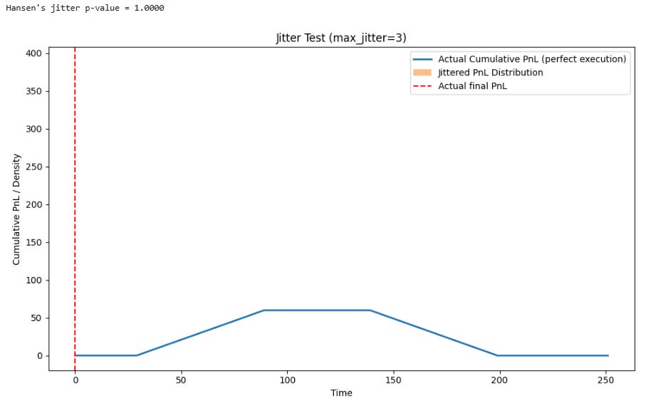
A tiny p-value in this test is a significant red flag. It indicates that perfect, instantaneous execution is critical to the strategy's profitability, a condition that never exists in live trading. This signals extreme execution fragility. Such strategies often have very low capacity and are highly sensitive to transaction costs.
A robust strategy should have its performance degrade gracefully, with its actual PnL curve staying within a reasonable band of the jittered PnLs, leading to a higher p-value. A failure here suggests the strategy's alpha is likely to be consumed entirely by transaction costs and implementation shortfall.
What we are looking is an actual final PnL close to the mean and a p-value close to 1. Large p-value (say p≈0.5 or higher) means that many of the jittered PnLs are as good as—or even better than—your perfect-execution PnL.