


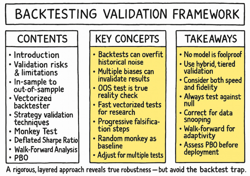
Table of contents:
Introduction.
Validation risks and backtest limitations.
The in-sample to out-of-sample transition.
A vectorized backtesting engine.
Techniques for strategy validation.
The null hypothesis benchmark.
Quantifying selection bias with the Deflated Sharpe Ratio.
Walk-Forward Analysis as a prelude to PBO.
The probability of backtest overfitting.
First layer to discard a model.
Before you begin, remember that you have an index with the newsletter content organized by clicking on “Read full story” in this image.

Introduction
You know, after more than a decade in this business, I've come to think of backtesting as the ultimate paradox of our profession. It's like being handed the top one lie detector in the world, only to discover it's been calibrated exclusively on your own personal brand of self-deception.
Let me tell you something about that moment—and every quant knows exactly which moment I'm talking about. You've been grinding through months of feature engineering, tweaking parameters, massaging data until your eyes bleed. Then suddenly, like lightning striking twice in the same place, you get the curve. That impossibly smooth, relentlessly ascending line that makes the S&P 500 look like amateur hour. Your heart starts racing because you think you've cracked the code. You've found the Holy Grail. The market's deepest secret has revealed itself to you personally.
But here's what nobody tells you in the intership:
That perfect equity curve is often the most expensive lesson you'll ever receive. It's market tuition paid in full.
The brutal truth? Your beautiful model hasn't discovered some hidden market inefficiency. It's become a savant at recognizing the wallpaper pattern in your historical data. Every idiosyncratic blip, every random walk drunk on a Tuesday afternoon, every correlation that existed purely by cosmic accident—your algorithm has memorized it all with the obsessive precision of a chess grandmaster studying a single game.
This is the curse of trading meets Murphy’s Law in a dark alley. You've essentially taught your model to be the world's most expensive parrot, capable of perfectly reciting the past but utterly mute when faced with tomorrow's surprises. The parameters have become so exquisitely tuned to historical noise that they've lost all ability to generalize. High variance, low bias—the classic overfitting signature that haunts every domain, but in finance, it comes with a special cruelty: it costs you money until you reach $0 in your account.
The psychological warfare is what really gets you. Confirmation bias whispers sweet nothings about your genius while the narrative fallacy helps you craft an elaborate story explaining why this random pattern actually represents some deep market truth. Before you know it, you've burned through every degree of freedom your data had to offer, fitting noise like it's signal, memorizing chaos like it's order.
The seductive thing about overfitting is that it doesn't announce itself with warning bells and flashing lights. Instead, it arrives disguised as brilliance and sometimes, your overfitted model works, indeed, it works in an incredible way during some periods of time—crazy, right!? However, the market has this delicious sense of humor and eventually, it doesn't just reject your overfitted model—it actively punishes it.
Many have studied this twist before. There are entire papers on this topic; here's a classic:

But the conclusion is always the same: The market, as always, gets the last laugh. And it's a laugh that echoes through every risk management meeting, every client call, every sleepless night spent wondering how something so beautiful in backtest could be so brutal in reality.
Validation risks and backtest limitations
Before any empirical results can be trusted, one must develop a deep and functional understanding of the inherent risks that can invalidate a backtest. These are not peripheral concerns but central flaws that can systematically corrupt the research process:
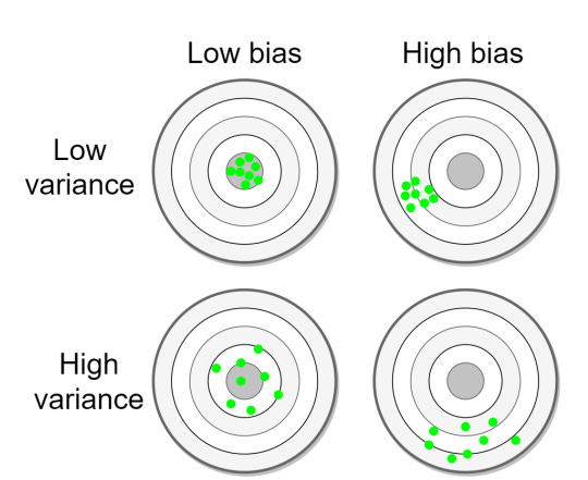
Backtest overfitting and the bias-variance tradeoff: This is the primary pathology of quantitative research. Formally, it represents a failure in managing the bias-variance tradeoff. A simple model—e.g., a long-term moving average crossover—may be too simple to capture the underlying market dynamic—high bias—while an overly complex model—e.g., a deep neural network with thousands of parameters or a rule-based system with dozens of conditions—can fit the in-sample data almost perfectly but will fail on new data—high variance. Overfitting occurs when a model is either excessively complex or has been selected from a vast universe of tested configurations.
The model begins to conform to the noise within the in-sample data rather than the underlying signal. The mathematical consequence is a model that exhibits low in-sample error but high out-of-sample error, indicating a failure of generalization.

Data snooping (aka multiple testing): This is a specific and statistically quantifiable form of overfitting. When a researcher evaluates a multitude of hypotheses on a single, finite dataset, the probability of discovering a seemingly significant result purely by chance escalates rapidly.
If one tests m independent, truly null hypotheses—e.g., strategies with no real edge—at a statistical significance level alpha, the probability of observing at least one result that passes this threshold by luck is given by the Family-Wise Error Rate (FWER):
\(\mathrm{FWER} = P(\text{at least one false positive}) = 1 - (1 - \alpha)^m \)A simple, though often overly punitive, method to control the FWER is the Bonferroni correction, which suggests using a stricter significance threshold of alpha′=alpha/m. However, while this reduces false positives, it also drastically increases false negatives, potentially causing one to discard genuinely good strategies. More advanced methods, discussed later, are required to properly manage this risk.
Survivorship bias: This data integrity issue arises when historical datasets exclude entities that have failed, been acquired, or been delisted. A backtest of a stock trading strategy on the current constituents of the S&P 500 index over a 20-year lookback period will be upwardly biased because the dataset implicitly excludes firms like Enron, WorldCom, or Lehman Brothers. The strategy, therefore, appears more profitable because its investment universe was retroactively cleansed of failures, a luxury not available in trading.
A famous historical example of risk miscalculation, partly due to looking at a set of surviving successful banks, was the 1998 collapse of Long-Term Capital Management, whose models failed to account for extreme events that were outside their historical—and survivorship-biased—dataset.
Look-ahead bias: This represents a temporal contamination of the simulation, where information that would not have been available at the time of a decision is erroneously included. It is a common and often subtle coding error. Beyond the classic example of using the closing price for a same-day trade, more subtle forms include:
Using a historical price series that has been adjusted for future stock splits and dividends can be a form of look-ahead bias if not handled carefully.
Normalizing a feature—e.g., scaling to have zero mean and unit variance—by calculating the mean and standard deviation over the entire dataset, and then using those normalized features in a point-in-time simulation, leaks information from the future into the past. The normalization must be done on a rolling basis using only data available up to that point.
Non-stationarity and concept drift: Financial markets are not statistically static systems. The underlying data-generating processes exhibit time-varying properties, a phenomenon quants call concept drift.
Regimes of low volatility can give way to periods of high volatility; correlations between assets can invert during a crisis; and phenomena like momentum or mean-reversion can strengthen, weaken, or disappear entirely based on macroeconomic conditions—e.g., interest rate regimes.
A strategy optimized on data from one market regime—for example, the post-2008 quantitative easing era—may be completely invalidated by a regime shift to quantitative tightening. An overfit strategy has not learned a general market law; it has learned the specific rules of a game that is no longer being played.
Transaction costs and slippage modeling: Backtests frequently abstract away from the frictional realities of market participation. Every trade incurs explicit costs—commissions, fees—and implicit costs—bid-ask spread, market impact. The market impact, or slippage, is the most difficult to model. It can be broken down into:
Delay slippage: The price change between when the signal is generated and when the order is actually placed in the market.
Market impact: The adverse price movement caused by the order itself, as it consumes liquidity. A common—though simplified—model for market impact is the square root model, which posits that the price impact is proportional to the square root of the order size relative to the average daily volume. A failure to model these costs with high fidelity can make a money-losing, high-turnover strategy appear to be a spectacular success.

The in-sample to out-of-sample transition
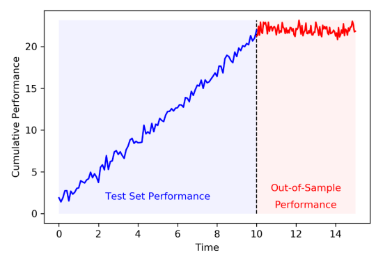
The central conflict of quantitative research, the very crucible where theory meets reality, crystallizes at a single, pivotal moment: when a strategy first encounters data it has not seen before. This is the transition from the in-sample (IS) period—the historical dataset used for discovery, calibration, and optimization—to the out-of-sample (OOS) period. The performance differential between these two periods is the ultimate, and often brutal, arbiter of a strategy's validity. An elegant in-sample equity curve is merely a hypothesis; the out-of-sample equity curve is the experimental result.
The degradation in performance from IS to OOS is not merely a matter of bad luck; it is a predictable consequence of the modeling process. Any financial time series contains two primary components:
A potentially persistent and exploitable signal.
A dominant, stochastic, and non-repeating noise component.
A flexible model, under the pressure of optimization, will inevitably learn a function that fits both. It learns to exploit the true signal—if one exists—while also contorting itself to perfectly map the specific, random undulations of the in-sample noise. When this overfit model is applied to OOS data, the signal component may still contribute positively, but the part of the model that memorized the in-sample noise is now actively detrimental, as it attempts to apply bygone patterns to a new and different random reality. The model's complexity, intended to capture signal, has instead become a source of error.
In the language of quants, this is a test of out-of-distribution generalization. Financial market data, however, presents a uniquely challenging form of this problem: The statistical properties of the data itself—the "rules of the game"—are in constant flux. Volatility, correlations, and the prevalence of trending or mean-reverting behavior all shift over time, creating distinct market regimes.
A strategy optimized for a low-volatility, trending bull market—one distribution—is almost certain to fail when confronted with a high-volatility, choppy bear market—a completely different distribution. Therefore, a model's ability to perform on OOS data is the only true measure of its worth, as it is the only test of its ability to generalize beyond the specific regime in which it was trained.
A vectorized backtesting engine
Before any advanced validation can occur, a researcher requires a robust and efficient backtesting engine. This mini lab will serve to determine whether it’s worth continuing with this line of research or, if not, it’s better to move on to another idea. The primary design consideration for such an engine is the trade-off between realism and speed.
Event-driven backtesters offer the highest fidelity. They operate as a state machine, processing market data tick-by-tick or bar-by-bar. They can manage a portfolio, handle complex order types—limit, stop, etc.—and model the order book dynamics. This makes them ideal for testing complex portfolio-level logic. However, their sequential nature makes them computationally intensive and slow, hindering rapid iteration during the research phase.
Vectorized Backtesters, in contrast, are designed for speed. This paradigm, central to scientific computing libraries like
pandasandnumpy, avoids explicit, slowfor-loops and instead applies mathematical operations to entire arrays—vectors or matrices—at once. In the context of a backtest, this means that calculations for returns, positions, and profit-and-loss are performed on the entire time series simultaneously. This approach provides a massive performance advantage, allowing a researcher to test thousands of strategy variations in the time it might take an event-driven engine to simulate one.
For the initial stages of research, where the goal is to quickly test many hypotheses and filter out unpromising ideas, the vectorized approach is vastly superior. The key is to construct the vectorized logic carefully to ensure accuracy, particularly in avoiding look-ahead bias and correctly modeling proportional transaction costs.
The following code snippet implements a standard recipe aka Backtester class. It is designed to be a foundational tool, consuming a time series of asset prices and a corresponding series of trading signals to generate a detailed performance analysis. The comments have been expanded to clarify the rationale behind each vectorized operation.
import numpy as np
import pandas as pd
from scipy.stats import skew, kurtosis
import matplotlib.pyplot as plt
import seaborn as sns
class Backtester:
"""
A high-performance, vectorized backtesting engine that consumes price and signal series
and computes a wide range of trading performance metrics.
This engine is designed for research and rapid iteration, leveraging
vectorized operations via pandas and numpy for high performance. It correctly
handles look-ahead bias and proportional transaction costs.
"""
def __init__(self,
price: pd.Series,
signals: pd.Series,
initial_capital: float = 100000.0,
transaction_cost: float = 0.001):
"""
Initializes the Backtester object.
Args:
price (pd.Series): Series of asset close prices, indexed by datetime.
signals (pd.Series): Series of trading signals (+1 for long, 0 for flat, -1 for short),
with the same index as the price series. The signal for a given
day T is assumed to be generated based on information available
before the close of day T.
initial_capital (float): The starting cash for the backtest.
transaction_cost (float): Proportional cost per trade (e.g., 0.001 for 0.1%).
"""
# Data Preparation and Validation
# Ensure data is sorted by date to prevent temporal errors
self.price = price.copy().sort_index()
# Align signals to the price index. This is crucial if the signal generation
# process creates a series with a different index. We fill any missing dates
# with a flat position (0), assuming no signal means no position.
self.signals = signals.reindex(self.price.index).fillna(0)
self.initial_capital = initial_capital
self.transaction_cost = transaction_cost
self.results = None # Will store the backtest results DataFrame
def run(self) -> pd.DataFrame:
"""
Executes the vectorized backtest.
This method calculates daily PnL by taking the element-wise product of the position
vector (determined by the previous day's signal) and the current day's return vector.
Transaction costs are incurred whenever the position changes.
"""
# 1. Calculate Market Returns
# The daily percentage change in price. The first value will be NaN, so we fill it with 0.
# This vector represents the return earned on day T if a position was held.
returns = self.price.pct_change().fillna(0)
# 2. Determine Positions (Crucial for avoiding look-ahead bias)
# The core of avoiding look-ahead bias is to use the signal from day T-1 to
# determine the position held throughout day T, which earns the return of day T.
# Shifting the signal series by one period forward achieves this vectorizedly.
# The first position will be NaN, so we fill it with 0.
positions = self.signals.shift(1).fillna(0)
# 3. Vectorized Profit & Loss Computation
# The gross PnL is the element-wise product of the positions vector and the returns vector.
# This single line calculates the daily PnL for the entire history.
pnl = positions * returns
# 4. Calculate Transaction Costs
# A trade occurs whenever the position changes. The `diff()` method calculates the
# change from the previous period (e.g., from +1 to -1 is a diff of -2).
# We take the absolute value as the size of the trade determines the cost, not its direction.
trades = positions.diff().abs()
# The cost is the value of the trade multiplied by the proportional transaction cost.
cost = trades * self.transaction_cost
# The net PnL is the gross PnL minus the associated transaction costs.
net_pnl = pnl - cost
# 5. Equity Curve Calculation
# The equity curve is the cumulative product of (1 + net daily PnL),
# which represents the compounding growth of the initial capital.
equity = (1 + net_pnl).cumprod() * self.initial_capital
# Store all intermediate and final results in a DataFrame for comprehensive analysis.
self.results = pd.DataFrame({
'Price': self.price,
'Signal': self.signals,
'Position': positions,
'Market Return': returns,
'Gross PnL': pnl,
'Trade Cost': cost,
'Net PnL': net_pnl,
'Equity': equity
})
return self.results
def performance_metrics(self, risk_free_rate: float = 0.0) -> dict:
"""
Computes an extensive set of trading performance metrics from the backtest results.
Args:
risk_free_rate (float): The annualized risk-free rate for calculating ratios like Sharpe.
This should be expressed as a decimal (e.g., 0.02 for 2%).
Returns:
A dictionary containing all key performance indicators (KPIs).
"""
if self.results is None:
raise RuntimeError("Backtest has not been run. Call .run() first.")
r = self.results['Net PnL']
equity = self.results['Equity']
total_return = (equity.iloc[-1] / self.initial_capital) - 1
n_periods = len(r)
annual_factor = 252 # Assuming daily data.
annualized_return = (1 + total_return) ** (annual_factor / n_periods) - 1
annualized_vol = r.std() * np.sqrt(annual_factor)
sharpe = (annualized_return - risk_free_rate) / annualized_vol if annualized_vol != 0 else np.nan
neg_returns = r[r < 0]
downside_vol = neg_returns.std() * np.sqrt(annual_factor) if not neg_returns.empty else 0
sortino = (annualized_return - risk_free_rate) / downside_vol if downside_vol != 0 else np.nan
peak = equity.cummax()
drawdown = (equity - peak) / peak
max_dd = drawdown.min()
calmar = annualized_return / abs(max_dd) if max_dd != 0 else np.nan
trade_count = int(self.signals.diff().abs().sum() / 2)
wins = r[r > 0]
losses = r[r < 0]
num_trades = len(wins) + len(losses)
win_rate = len(wins) / num_trades if num_trades > 0 else np.nan
profit_factor = wins.sum() / abs(losses.sum()) if losses.sum() != 0 else np.nan
return {
'Total Return': total_return,
'Annualized Return': annualized_return,
'Annualized Volatility': annualized_vol,
'Sharpe Ratio': sharpe,
'Sortino Ratio': sortino,
'Maximum Drawdown': max_dd,
'Calmar Ratio': calmar,
'Trade Count': trade_count,
'Win Rate': win_rate,
'Profit Factor': profit_factor,
'Skewness': skew(r, nan_policy='omit'),
'Kurtosis': kurtosis(r, nan_policy='omit')
}
def plot_results(self):
"""Generates a standard performance tear sheet plot."""
if self.results is None:
self.run()
fig, axes = plt.subplots(3, 1, figsize=(14, 15), sharex=True)
fig.suptitle('Strategy performance analysis', fontsize=16)
# Plot 1: Equity Curve and High Water Mark
axes[0].plot(self.results['Equity'], label='Equity curve', color='blue', lw=2)
axes[0].plot(self.results['Equity'].cummax(), label='High water mark', color='green', linestyle='--', lw=1)
axes[0].set_title('Equity curve')
axes[0].set_ylabel('Portfolio value ($)')
axes[0].legend(loc='upper left')
axes[0].grid(True)
# Plot 2: Price Series with Positions
axes[1].plot(self.results['Price'], label='Asset Price', color='black', lw=1)
axes[1].set_title('Price and trading positions')
axes[1].set_ylabel('Price')
ax2_twin = axes[1].twinx()
ax2_twin.fill_between(self.results.index, 0, self.results['Position'], where=self.results['Position'] > 0, color='green', alpha=0.2, label='Long Position')
ax2_twin.fill_between(self.results.index, 0, self.results['Position'], where=self.results['Position'] < 0, color='red', alpha=0.2, label='Short Position')
ax2_twin.set_ylabel('Position')
ax2_twin.legend(loc='upper right')
axes[1].legend(loc='upper left')
axes[1].grid(True)
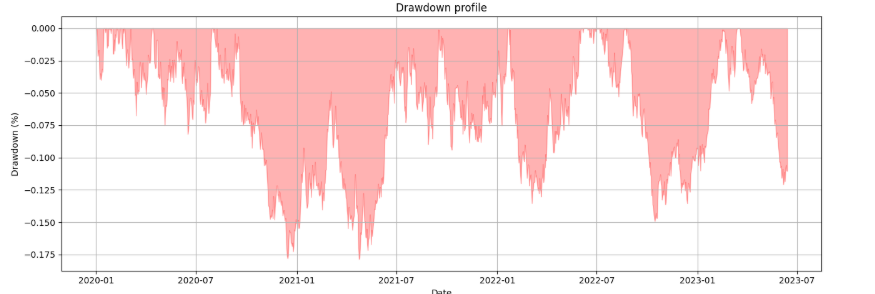
# Plot 3: Drawdown Series
drawdown_series = (self.results['Equity'] - self.results['Equity'].cummax()) / self.results['Equity'].cummax()
axes[2].fill_between(drawdown_series.index, drawdown_series, 0, color='red', alpha=0.3)
axes[2].set_title('Drawdown profile')
axes[2].set_ylabel('Drawdown (%)')
axes[2].set_xlabel('Date')
axes[2].grid(True)
plt.tight_layout(rect=[0, 0, 1, 0.96])
plt.show()Using the Backtester class requires providing price and signal data. The following demonstrates a typical workflow, from generating a simple moving average crossover strategy to evaluating its performance and interpreting the output.
# 1. Generate Synthetic Data
np.random.seed(42)
price_series = pd.Series(100 + np.random.randn(252 * 5).cumsum(),
                         index=pd.to_datetime(pd.date_range('2020-01-01', periods=252 * 5)))

# 2. Create a Simple Trading Strategy Signal
fast_ma = price_series.rolling(window=30).mean()
slow_ma = price_series.rolling(window=90).mean()
signal_series = pd.Series(np.where(fast_ma > slow_ma, 1, -1), index=price_series.index).fillna(0)

# 3. Instantiate and Run the Backtester
bt = Backtester(price=price_series,
                signals=signal_series,
                initial_capital=100000,
                transaction_cost=0.001)
bt.run()
metrics_dict = bt.performance_metrics()

# 4. Analyze Results
print("--- Performance Metrics ---")
metrics_series = pd.Series(metrics_dict)
print(metrics_series.to_string(float_format="{:.4f}".format))

bt.plot_results()
How would we interpret its output?
Sharpe ratio: The workhorse metric. A value > 1 is generally considered good, > 2 is very good. However, as we will see, it can be misleading.
Sortino ratio: A refinement of the Sharpe. A Sortino Ratio significantly higher than the Sharpe Ratio suggests that the strategy's volatility is skewed to the upside—a desirable trait. A lower Sortino suggests painful downside volatility.
Maximum drawdown: A critical measure of risk. This represents the worst peak-to-trough decline in portfolio value. It gives a gut-check sense of the most pain the strategy would have inflicted. A drawdown > 20% is often considered high for most investors.
Calmar ratio: Annualized return / Max drawdown. It measures return relative to the worst-case loss. A Calmar > 1 is decent, > 3 is excellent. It is particularly useful for conservative investors.
Skewness: Measures the asymmetry of returns. A negative value (< -0.5) is a red flag, indicating a tendency for large, negative outliers—crashes. Positive skew is desirable.
Kurtosis: Measures the tailedness of the return distribution. A high value—e.g., > 3, which is the kurtosis of a normal distribution—indicates fat tails, meaning extreme events—both positive and negative—are more likely than a normal distribution would suggest. This is a crucial indicator of hidden risk.
This backtesting engine provides the necessary quantitative outputs. It tells us what happened. But this is not what we want to know. We want to know if our system would survive in the future!
Also, look how interesting! These are the results of testing the previous average crossover on random data. It doesn't leave you with a weird, strange feeling, like something's wrong, right?

I don't know about you, but I'd be pretty puzzled about paying a PM if the backtest of a crossover of averages on random data yielded these results... But okay, let’s continue, the crucial subsequent step is to determine why it happened and whether the observed performance is statistically robust or merely an artifact of luck.
Techniques for strategy validation
With a functional backtester, we can now progress to the core task: stress-testing the strategy. The following techniques form an integrated framework for falsification. They are designed to be applied sequentially, each posing a more difficult hurdle for the strategy to clear. A strategy that survives this gauntlet is one in which we can have a moderate degree of evidence-based confidence.
This is the first step. In the next series of articles, we'll explore more complex tools that provide more evidence about the reliability of a strategy, or whether you're just throwing your money away.
The null hypothesis benchmark
The term traces back to Burton G. Malkiel’s 1973 classic A Random Walk Down Wall Street, where he quipped that a blindfolded monkey throwing darts at the stock listings could select a portfolio that would do just as well as one selected by experts. This colorful image highlights the Efficient Market Hypothesis, arguing that markets are so efficient that professional stock-pickers struggle to consistently beat a random selection.
The most fundamental question to ask of any backtest is: Is this result distinguishable from pure, dumb luck? Before comparing a strategy to benchmarks, we must first demonstrate that it is superior to a legion of monkeys—for this reason it is known as The Monkey Test—randomly placing trades. This test, often called a Monte Carlo permutation test, establishes a baseline of performance under the null hypothesis (H_0) that the strategy's logic has no predictive power.
The core idea is to generate a large number, N, of random trading signal series. These series should preserve certain characteristics of the original strategy's signals, most importantly the trading frequency or the proportion of time spent in the market. A more advanced approach involves using a block bootstrap on the original signals, which preserves some of the autocorrelation structure present in the original strategy, making for a more challenging null hypothesis. We then run a backtest on each of these N random strategies to generate a distribution of a chosen performance metric—e.g., the Sharpe Ratio. This distribution represents the range of outcomes one could expect to achieve by chance alone.
The performance of our actual strategy, SR_actual, is then compared to this distribution. The p-value of the test is the fraction of random strategies that achieved a Sharpe Ratio greater than or equal to our actual strategy's Sharpe Ratio.
A low p-value (p<0.05) suggests that it is statistically unlikely that the strategy's performance was a result of random chance. Let’s code it:
def run_monkey_test(backtester_instance, n_monkeys=1000):
    """
    Runs a Monte Carlo simulation with random trading signals to test
    the statistical significance of a strategy's performance.

    Args:
        backtester_instance (Backtester): An instance of the Backtester class, already
                                          initialized with price data and the actual strategy signals.
        n_monkeys (int): The number of random simulations to run.

    Returns:
        A tuple containing:
        - The actual strategy's Sharpe Ratio.
        - A list of Sharpe Ratios from the random strategies.
        - The calculated p-value.
    """
    if backtester_instance.results is None:
        backtester_instance.run()
    actual_metrics = backtester_instance.performance_metrics()
    actual_sharpe = actual_metrics['Sharpe Ratio']

    original_signals = backtester_instance.signals
    n_periods = len(original_signals)
    signal_proportions = original_signals.value_counts(normalize=True)

    random_sharpes = []
    print(f"Running simulation with {n_monkeys} random strategies...")

    for i in range(n_monkeys):
        random_signals_array = np.random.choice(
            signal_proportions.index,
            size=n_periods,
            p=signal_proportions.values
        )
        random_signals = pd.Series(random_signals_array, index=original_signals.index)

        monkey_bt = Backtester(
            price=backtester_instance.price,
            signals=random_signals,
            initial_capital=backtester_instance.initial_capital,
            transaction_cost=backtester_instance.transaction_cost
        )
        monkey_bt.run()
        monkey_metrics = monkey_bt.performance_metrics()
        random_sharpes.append(monkey_metrics['Sharpe Ratio'])

    random_sharpes = np.array(random_sharpes)
    p_value = np.sum(random_sharpes >= actual_sharpe) / n_monkeys

    return actual_sharpe, random_sharpes, p_value

# Main
actual_sharpe, random_sharpes_dist, p_value = run_monkey_test(bt, n_monkeys=2000)
The resulting plot provides an immediate visual assessment of the strategy's merit. If the red line—the actual strategy's performance—is deep within the distribution of random results, it signifies that a monkey throwing darts at a board could likely have achieved a similar or better outcome. If, however, the strategy's performance lies in the far-right tail of the distribution, corresponding to a low p-value, we can reject the null hypothesis and conclude that the strategy's performance is statistically significant relative to random chance.
In this case, the strategy surpasses chance, which has another interpretation:
Even completely random strategies can obtain good results and make you believe that you have alpha.
Due to the previous reason, passing this test is a necessary, but not sufficient, condition for a strategy to be considered valid. It is the first and most basic hurdle.
Next we will see why this test, as it is presented, is not sufficient.

Quantifying selection bias with the Deflated Sharpe Ratio
The Monkey Test guards against a single strategy being lucky. Data snooping addresses a more insidious problem: the researcher's own process of selection. If a researcher tests n plausible strategy variations, the act of selecting the best performing variation introduces a significant positive bias. The performance of the chosen strategy is no longer a random draw from the distribution of all possible outcomes; it is the maximum.
This selection bias must be quantified and corrected for. The Deflated Sharpe Ratio (DSR) is a metric designed to estimate what the Sharpe Ratio would be after removing the inflationary effect of multiple testing.
The DSR deflates an observed Sharpe Ratio, based on the number of trials (m), the length of the time series (T), and the skewness and kurtosis of the returns. The full formula is complex, but a simplified version is given by:
Where Phi-1 is the inverse CDF of the standard normal distribution, and Var(widehatSR) is the variance of the Sharpe Ratio estimate itself, which can be approximated as:
Here, hatmu3 and hatmu4 are the sample skewness and kurtosis of the returns. The DSR essentially calculates the threshold for statistical significance given m trials and then reports a Sharpe of zero if the observed Sharpe is below this threshold.
Let’s code it:
from scipy.stats import skew, kurtosis, norm

def deflated_sharpe_ratio(estimated_sr: float,
                          returns: pd.Series,
                          num_trials: int) -> float:
    """
    Compute the Deflated Sharpe Ratio (DSR), dropping NaNs
    and omitting them in the moment calculations.
    """
    r = returns.dropna()
    T = len(r)
    if T < 2:
        return np.nan

    μ3 = skew(r, bias=False, nan_policy='omit')
    excess_kurt = kurtosis(r, fisher=True, bias=False, nan_policy='omit')
    μ4 = excess_kurt + 3.0

    var_sr = (1.0 / (T - 1)) * (
        1
        - μ3 * estimated_sr
        + ((μ4 - 1) / 4.0) * estimated_sr**2
    )
    if var_sr <= 0:
        return np.nan
    σ_sr = np.sqrt(var_sr)

    z1 = norm.ppf(1 - 1.0 / num_trials)
    z2 = norm.ppf(1 - 1.0 / (num_trials * np.e))
    τ = (1 - μ3) * z1 + μ3 * z2

    return (estimated_sr - τ * σ_sr) / σ_sr

# Main
returns = bt.results['Net PnL']
cleaned = returns.dropna()
sample_sr = cleaned.mean() / cleaned.std(ddof=1)
m = 100
dsr = deflated_sharpe_ratio(sample_sr, returns, num_trials=m)

print(f"Sample Sharpe: {sample_sr:.4f}")
print(f"Deflated Sharpe Ratio (m={m}): {dsr:.4f}")
That negative DSR means that, once you account for having tried 100 different versions of your strategy, your observed Sharpe actually under‐performs the threshold you’d expect to clear even by pure luck—now DSR is negative. In other words, picking the best Sharpe out of 100 noisy backtests typically yields around a 0.03 daily Sharpe just by chance—so it falls below that noise floor.
In a professional quant this would send you back to the drawing board:
A backtest Sharpe of 0.39 looks fine until you realize—thanks to DSR—you haven’t actually demonstrated anything above random noise.
A process that tests a few, well-motivated ideas is far more likely to produce a strategy with a positive DSR than a brute-force process that tests everything. This metric is an antidote to the problem of finding needles of alpha in a haystack of noise and then claiming the needle is special without acknowledging the size of the haystack.
This isn't starting to look as pretty as the backtest and monkey test made it seem. Let's move on!
Walk-Forward Analysis as a prelude to PBO