

[WITH CODE] Data transformations: Data shape and predictive features
Alternative data shape transformation

Table of contents:
Introduction.
Data-Shape transformation.
Identifying the risks and limitations.
Data shape transformations for predictive features.
State-space approach.
Dynamic benchmark neutralization.
Stochastic trend removal via cointegration.
Multiscale isolation approach.
Bounded state encoding.
Before you begin, remember that you have an index with the newsletter content organized by clicking on “Read the newsletter index” in this image.

Introduction
Imagine that a team downloads a price series, defines a target, applies a transformation, and moves on to signal design, model fitting, validation, and execution. That sequence looks efficient. However, the transformation of the data is is the first act of model construction.
That is why data-shape transformation sits at the true front line of feature engineering. The problem is whether the operator used to create that series preserves the economic structure that generates predictive edge. A feature can look impeccable under statistical diagnostics and still be useless in live trading. It can pass every formal test of stability while removing the component that contained the alpha.
This article examines that hidden fault line. It argues that data-shape transformation must be treated as a structural modeling choice rather than a preprocessing convenience. We will identify the main risks introduced by transformation operators, explain how they distort the topology of predictive information, and then study five targeted transformations designed for distinct market nuisances: state-space innovations, rolling benchmark residuals, cointegration spreads, multiscale Haar details, and rolling range positions. The objective is not to make features look cleaner. The objective is to ensure that the shape of the data remains faithful to the market mechanism the model is supposed to learn.
Every transformation enforces a decision about relevance. It selects one part of the market path and suppresses another. It may emphasize short-horizon variation, eliminate common drift, compress local extremes, or redefine the position of the current price relative to its recent history. Before any model is trained, the researcher has already imposed a theory of what matters.
By the way, you can go deeper in this topic by exploring this paper.

That choice is decisive because financial data are layered. A single price series contains slow structural movement, temporary dislocations, benchmark comovement, volatility clustering, and random noise at the same time. A predictive model is never interested in all these layers equally. It depends on a narrow component that matches the strategy horizon and economic logic. The transformation either isolates that component or removes it.

Data-Shape transformation
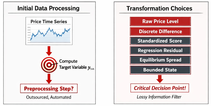
The starting phase of feature engineering contains a severe trap because it masquerades as a trivial data processing step. A quant team downloads a time series of prices, computes a target variable, and faces the decision of whether the predictive model should ingest the raw level, a discrete difference, a standardized statistical score, a regression residual, an equilibrium spread, or a bounded state variable. The standard academic and industry reflex is to treat this decision as a technical prerequisite, often labeled preprocessing or data normalization. That classification is a mistake.
In many pipelines, this step is outsourced to data engineers or automated via standard library defaults before the alpha researchers even begin their core modeling. This assumes that data transformation is a lossless translation of information. It is not. Once a specific transformation is applied to the raw time series, the researcher has declared what specific variation in the market path constitutes actionable information and what variation constitutes noise. If the chosen transformation is misaligned with the economic mechanism the strategy intends to exploit, the resulting model can exhibit perfect statistical behavior while remaining economically blind.
In our domain, this situation is unforgiving because the price is a cumulative, high-memory object. It aggregates historical microstructure shocks, macroeconomic regime shifts, discrete splits in volatility, slow reallocations of institutional capital, structural risk premia, and continuous benchmark movements.
A raw price level carries a massive amount of historical baggage that the short-term or medium-term target variable is invariant to. Assume the core research problem is to predict the magnitude and direction of a short-horizon log return yt+h. The actual feature matrix the learning algorithm receives is rarely the raw price pt. Instead, the model ingests a transformed object xt = T(Ft), where Ft represents the filtration generated by the history of prices and exogenous covariates up to time t. The selection of the transformation operator T is the actual front line of the research design. This operator dictates whether the vector xt represents a local surprise, a relative displacement, a structurally bounded state, etc.
Identifying the risks and limitations
The risk surface introduced by the operator T is broader and more destructive than standard statistical literature admits. Researchers frequently inherit standard transformation recipes without interrogating their geometric implications or their effect on the data topology. They compute discrete log returns rt = \ln(pt) - \ln(pt-1) because financial libraries expect stationary inputs. They build rolling z-scores because the resulting chart oscillates symmetrically around zero and fits neatly into the activation functions of deep neural networks. These choices impose heavy structural assumptions. A standard return calculation deletes the absolute price level and the cumulative memory of the path. A residual calculation deletes the variance explained by the specified reference model.
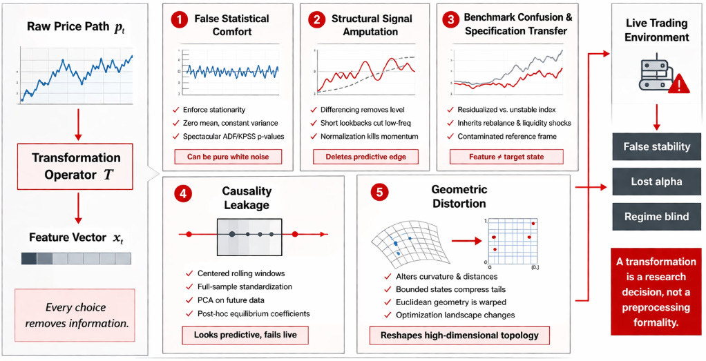
The first specific risk is false statistical comfort. A transformed time series can be manipulated to exhibit perfect weak-sense stationarity, zero mean, and constant variance, while simultaneously failing to express any tradable market state. Any researcher can run an Augmented Dickey-Fuller or KPSS test, achieve a spectacular p-value, and incorrectly assume the feature is ready for predictive modeling. Extracting white noise from a time series guarantees stability, but white noise contains zero predictive alpha. The researcher has converted the price into a stable sequence that is devoid of economic value.
The second risk is structural signal “amputation”. A transformation can neutralize the exact slow-moving component that carried the predictive edge. This failure mode occurs when researchers impose rigid discrete differencing, rolling normalization, or arbitrary short lookback windows without first establishing the exact holding period the systematic strategy is designed to exploit. If a macro trend-following strategy relies on three-month momentum, applying a 5-day rolling z-score to the input features will delete the low-frequency eigenvalue that the model requires to identify the trend.
The third risk is benchmark confusion and specification transfer. When a transformation operator incorporates a secondary series—such as a benchmark ETF, a sector index, or a paired asset—the resulting feature inherits the specification risk of that external asset. A regression residual is only valid if the variable against which it is residualized represents a stable economic factor. If a researcher isolates a tech stock by residualizing it against the QQQ index, and the index undergoes a massive constituent rebalance or suffers a liquidity shock, the resulting feature vector will exhibit severe volatility that has nothing to do with the target stock’s idiosyncratic state. The feature becomes contaminated by the reference frame.
The fourth risk is causality leakage. This is the most common fatal error in systematic trading. When the transformation relies on parameters estimated using information outside the filtration Ft, the feature becomes predictive in the research environment and false in the production environment. Using centered rolling windows, applying Principal Component Analysis eigenvectors derived from the full target matrix, computing full-sample mean vectors for standardization, or extracting post-hoc equilibrium coefficients creates a matrix that cannot exist in live trading. Forward-looking bias is adept at hiding within the scaling constants of data-shape transformations.
The fifth risk is geometric distortion. This transformation alters local curvature, variance persistence, variance clustering, and the relative distance metric of excursions. Consider a neural network optimizer relying on Euclidean distance to compute gradients. Mapping a log-normal price path into a bounded state space between zero and one forces the distance metric near the boundaries to behave differently from the distance metric in the center of the distribution. A raw price move that represents a massive four-standard-deviation tail event might only translate to a 0.01 shift in the bounded feature space if the state was already sitting at 0.98. Extracting a state space model collapses a continuous smooth drift into a localized sequence of forecast errors clustered around zero. This alters the fundamental definition of what a market burst represents to the downstream algorithm.
The conflict between raw data and transformed geometry culminates in a specific, observable failure in the research lifecycle. A model is built on a transformed feature set. The initial teardown looks immaculate. The in-sample backtest “demonstrates” it works. The cross-validation metrics are stable across distinct market regimes. The feature importance vectors are dense and logical. The Sharpe ratio appears robust across multiple chronological subsamples, and the drawdowns are well contained.
Then… the model is advanced to paper trading or live execution, and the predictive relationship collapses. The alpha decay instantaneous. The post-mortem analysis reveals that the algorithm never learned the underlying market mechanism. The optimization process learned the geometry introduced by the transformation operator T. It fit itself to sample-specific trend removal artifacts, spurious benchmark dependencies, bound-rejection behavior dictated by rolling window mechanics rather than market participants, and local scaling normalization patterns that possessed no forward-looking stability.

Data shape transformations for predictive features
If the strategy is engineered to trade benchmark-relative mispricing, then the absolute market benchmark exposure is the primary nuisance structure. If the strategy capitalizes on statistical arbitrage and pair reversion, the common stochastic trend is the primary nuisance structure. If the strategy dictates short-horizon momentum reactions, slow multi-month macroeconomic drift is the primary nuisance structure. If the strategy operates as a local-state mean-reversion classifier, the absolute nominal price level is the primary nuisance structure.
This perspective enforces a precise operational taxonomy of data-shape transformations. The state space algorithm eliminates predictable local trends governed by state-space transition matrices, leaving the prediction surprise. The rolling_regression_residual algorithm eliminates time-varying benchmark exposure, yielding a relative-value deviation vector. The cointegration_spread algorithm eliminates common stochastic drift based on equilibrium vector autoregression logic, resulting in a stationary spread conducive to error-correction modeling. The haar_detail_same_length algorithm eliminates low-frequency power at a selected scale, leaving a targeted multiscale shock component. The rolling_range_position algorithm eliminates absolute nominal levels and local variance scaling, yielding a bounded coordinate variable.
These five methods represent interventions designed to blind the model to specific, targeted market nuisances. However without the right measures, the same mistakes could continue in some of them. Now that you’re aware of them, we can move forward.
State-space approach
The first targeted transformation is the state-space. In technical literature, this is defined as the one-step-ahead prediction error derived from a local linear trend state-space model. This transformation alters the time-series geometry by removing the exact variation that the internal state estimate already expects the system to produce at time t. This isolation mechanism is required when the raw log-price is cumulative, exhibiting a smooth drift that masks the actual high-frequency surprise component necessary for short-horizon prediction.
The formulation relies on setting up the observed log-price yt as the output of a local linear trend model. The system requires an observation equation and state transition equations:
Here, the unobserved latent state consists of the level μt and the slope βt. The disturbances εt, ηt, and ζt are mutually independent Gaussian white noise processes governing the measurement error, the level shift, and the slope shift. The state space model operates recursively. Given the filtration up to t-1, it produces the optimal linear one-step-ahead prediction E[yt | Ft-1]. The feature we extract is the sequence vt:
It is crucial to understand that vt represents the precise segment of the current price movement that could not be predicted by the prior dynamic state. In the context of algorithmic trading, this means the feature measures orthogonal surprise rather than raw directional motion.
The rationale for this transformation is embedded in market microstructure. A high-frequency algorithm processing order flow must differentiate between a market that ticks upward at a steady, anticipated velocity and a market that prints an identical upward tick against a declining latent trend. The nominal difference yt -yt-1 will record an identical positive value in both scenarios. The state space vt will output a minor value for the first scenario and a massive positive value for the second. Innovation-based feature engineering forces the learning algorithm to respect the conditional context of the regime.
def state_space(price_series: pd.Series) -> pd.Series:
    """
    Extracts the one-step-ahead forecast error from a local linear trend
    state-space model.
    """
    lp = price_series.rename("log_price")

    model = UnobservedComponents(lp, level="local linear trend")
    result = model.fit(disp=False)

    space = pd.Series(
        result.filter_results.forecasts_error[0],
        index=lp.index,
        name="state_space",)

    space.iloc[0] = np.nan
    return space
However, the researcher must decide if local drift should be neutralized. For execution timing, short-term liquidity provision, and algorithmic burst-detection, neutralizing drift is necessary. Utilizing vt ensures the resulting feature matrix is robust across shifting volatility regimes because the state-space covariance matrices adapt to changing latent slopes. The downstream classifier is thus relieved of the computational burden of discovering that adaptation matrix from raw inputs.
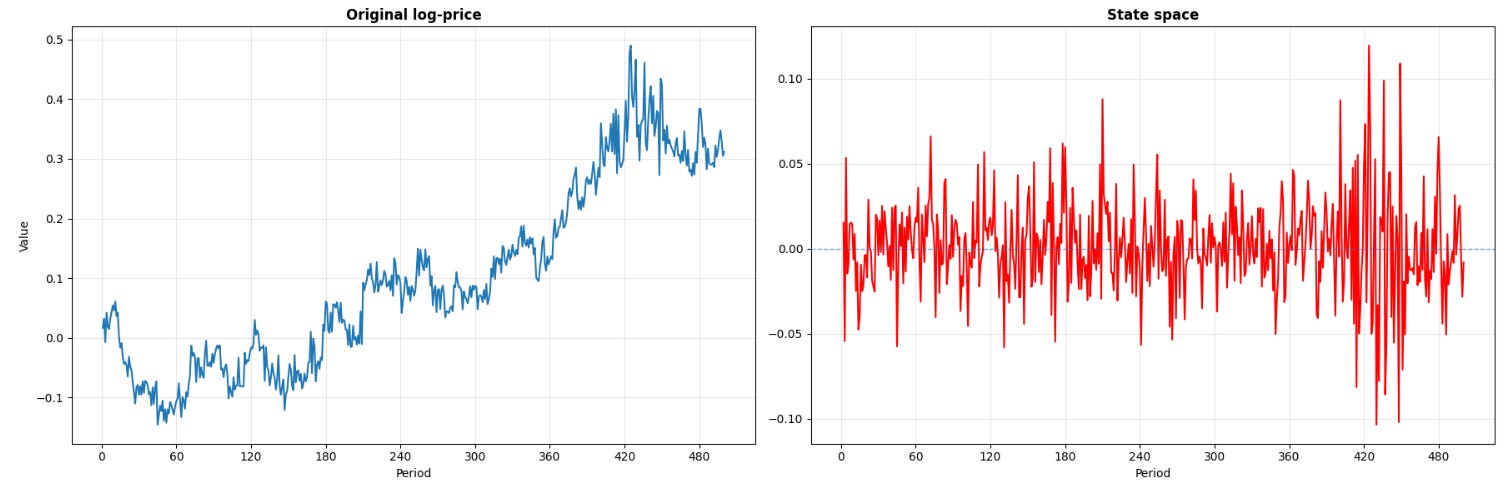
The primary failure mode of this transformation is specification error, which occurs when the assumed dynamics of the state-space model fail to map onto the conditions of the asset’s microstructure. The standard local linear trend model relies on continuous Gaussian diffusion. If the true data generation process is instead dominated by discrete Poisson jumps—such as overnight gaps, scheduled FOMC macroeconomic releases, or sudden liquidity vacuums—the linear Gaussian assumptions break down. When a structural price jump occurs, the linear filter cannot snap to the new regime. Instead, it lags, requiring multiple timesteps for the state space gain matrix to fully correct the latent state components. During this structural catch-up phase, the sequence vt will output an artificial cluster of large values. These values no longer represent an orthogonal market surprises but a deterministic filter correction error.
Researchers are tempted by the aesthetic stability of the a posteriori residual, often extracted via two-sided smoothing algorithms provided by default in many statistical libraries. Because these smoothers utilize future price information from t+1 to T to optimize the state estimate at time t, utilizing them injects terminal forward-looking leakage into the feature matrix. The resulting in-sample backtest will generate flawless, profitable metrics, while the live production system will bleed money.
Dynamic benchmark neutralization
The second transformation points to a different geometric annoyance known as time-varying external beta. The label is the rolling Ordinary Least Squares residual. In systematic portfolio management, this is recognized as the dynamic hedge residual. The core logic dictates that the variance of the target asset yt is contaminated by the variance of an external factor xt, which could represent a sector ETF, a broad index future, or a principal component basket. To model the asset’s idiosyncratic state, the researcher must regress the asset against the reference factor and isolate the residual error.
The model specifies:
Because the relationship between financial assets is never static, αt and βt cannot be estimated over the full sample. They must be approximated over a rolling window of length w. The parameter vector is computed utilizing the local design matrix Xt-w+1:t. The resulting transformed feature is the out-of-sample or end-of-sample deviation:
This specific subtraction is geometrically distinct from subtracting simple returns or computing a ratio. The dynamic residual projects the asset into the null space of the benchmark over the specified lookback window. The output geometry abandons the absolute coordinate system and adopts a relative, benchmark-neutral coordinate system.
def rolling_regression_residual(
    price_series: pd.Series,
    benchmark_series: pd.Series,
    window: int = 80,) -> pd.Series:
    """
    Computes the dynamic rolling residual of the asset relative to the benchmark.
    """
    y = price_series.rename("log_price")
    x = benchmark_series.rename("log_benchmark")

    X = sm.add_constant(x)
    result = RollingOLS(y, X, window=window).fit()
    params = result.params

    fitted = params["const"] + params["log_benchmark"] * x
    residual = (y - fitted).rename(f"rolling_regression_residual_{window}")

    return residual
In algorithmic trading, raw price vectors deceive predictive models by presenting sector-wide beta expansion as idiosyncratic momentum. A single equity instrument may display severe overbought technical geometry when the underlying condition is uniform sector strength. A cryptocurrency token may exhibit severe downward drift when the entire beta complex is repricing. Feeding raw prices into a deep neural network forces the network to allocate hidden layers to the task of inferring the benchmark matrix and computing the subtraction. By passing ût, the transformation executes the subtraction analytically, presenting the network with the pure, actionable relative-value deviation.
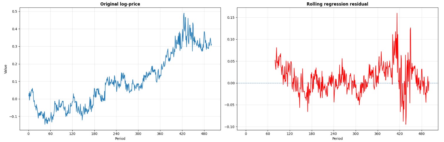
The geometric shift transforms a trend-dominated price path into a sequence that continually crosses zero, widening when the beta relationship degrades and compressing when the hedge is tight. This sequence describes relative-value dislocations that are primed for statistical arbitrage.
The implementation contains a critical stability trade-off governed by the window parameter w. A minimal window length allows the matrix inversion (XTX)-1 to adapt to microstructural shifts in beta, but exposes the parameters to severe estimation noise and matrix ill-conditioning. A maximum window length stabilizes the eigenvalue structure of the covariance matrix but renders the hedge ratio unresponsive to macroeconomic events.