


Table of contents:
Introduction.
Limitations and risks when parameterizing models.
Parametrization challenges.
The illusion of the global optimum.
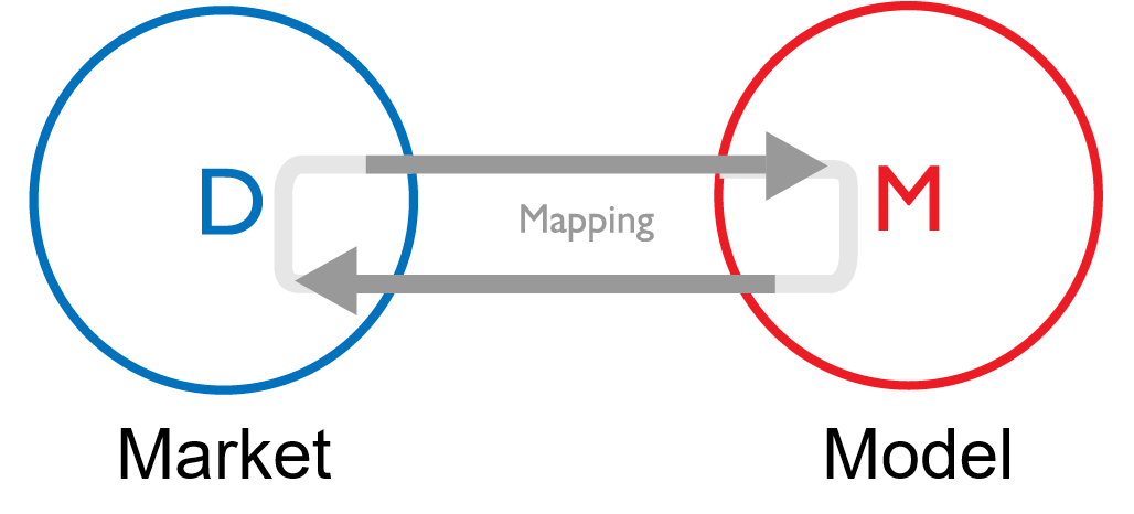
The foundational model.
Walk-forward framework.
Rolling windows with embargo.
Backtesting helpers.
Executing the Walk-Forward process.
K-Means clustering to identify parameter regimes.
Final selection of parameters.
Before you begin, remember that you have an index with the newsletter content organized by clicking on “Read full story” in this image.

Introduction
I want to start by saying that the key is in the data, not in the model or its parameters. Therefore, if your data is garbage, no matter how much you parameterize it, the results will still be garbage. If you parameterize a model, it's to fine-tune something that already works. Period.
Knowing that, we can proceed. The genesis of a strategy is often an elegant, compelling concept. This concept is then meticulously translated into a computational model, an architecture of logic replete with parameters. The immediate, almost instinctual, drive is to calibrate these parameters to what appears to be perfection, right?
This is the foundational dilemma of optimization: we are armed with a model, a finite history of market data, and an overwhelming incentive to tune the model's parameters to sculpt the most aesthetically pleasing performance curve on that historical data.
We can formalize this endeavor as a constrained optimization problem. Let S represent our trading strategy, which is a function of a parameter vector θ.
This vector θ belongs to a predefined parameter space Θ, such that:
Given a historical dataset D, which is a time-ordered sequence of market observations, our objective is to identify a specific parameter vector θ* that maximizes a chosen performance metric, our objective function f(⋅).
This function quantifies the desirability of a strategy’s outcome, encompassing metrics such as total return, Sharpe ratio, Calmar ratio, or other measures of risk-adjusted profitability. The mathematical representation of this search is:
This equation is the wet dream for quantitative analysts. It presents a deceptively linear path to success: discover the optimal parameters on past data, deploy, and profit. The procedure appears robust. Let's consider a simple model that depends on a single parameter: the lookback window N. The process involves iterating through all plausible integer values of N within a given range. For each candidate value, a backtest is executed on the historical dataset D. The objective function f(⋅) is computed for each resulting equity line, and the value of N that yields the maximum score is anointed as N.
To know more and see another example check this:
The outcome is frequently a spectacular equity curve, a testament to the power of optimization. It is a process that is algorithmically clean, mathematically precise, and almost invariably, a prelude to failure.
Limitations and risks when parameterizing models
The principal hazard, the latent variable in this deterministic optimization, is overfitting, a term more formally known in statistics as curve-fitting. This phenomenon occurs when a model, through the optimization process, becomes so intricately calibrated to the specific noise, outliers, and random fluctuations inherent in the training dataset that it forfeits its ability to generalize to new, unseen data. The distinction is analogous to that between genuine learning—internalizing the underlying principles of a system—and rote memorization. A model that has merely memorized the past is brittle; it has learned a specific sequence, not a general pattern.
Let's define this more rigorously. The performance we observe on our historical, in-sample data D gives us the in-sample error, Ein. The true test of a model, however, is its performance on future, out-of-sample data, which yields the out-of-sample error, Eout. The goal of any robust modeling process is to find a model that minimizes Eout. The process of maximizing performance on D is equivalent to minimizing Ein. Overfitting is the condition where we have successfully minimized Ein but at the cost of increasing Eout.
By selecting the single best parameter set θ*, we are, by construction, selecting the configuration that most effectively exploited the statistical artifacts of our specific historical sample. The risk is that this optimal performance is not a consequence of the model's intrinsic predictive power (its edge), but rather a statistical illusion born from data dredging. When this overfitted model is deployed into the live market, it confronts a data distribution for which it was not trained, and its performance rapidly and often decouples from the backtest.
The pivotal conflict that animates this entire analysis is this paradox: a strategy's viability is contingent on parameters that require optimization, yet the conventional act of optimization itself introduces a risk of self-deception and future failure. The central question becomes: how do we calibrate our model without rendering it a historical specialist, perfectly adapted for a market that no longer exists?

Parametrization challenges
I like to think of models as a deeper appreciation of the nature of their parameters. For example, in a breakout model, the parameter N (the lookback window) is the lens through which the model perceives market dynamics. A small N yields a model with high sensitivity, attuned to short-term oscillations, but also susceptible to being misled by market noise (high variance). A large N produces a model that is more inert, filtering out minor fluctuations to focus on established, durable trends, but at the risk of being slow to react to major structural shifts (high bias). Neither approach is axiomatically superior; their efficacy is regime-dependent. The purpose of parametrization is to endow our model with the requisite flexibility to adapt its logic.
The first practical obstacle is the dimensionality and topology of the parameter space θ. Our simple model has one dimension, N. Most institutional strategies, however, are multiparametric, involving thresholds for entry, rules for exit (profit targets, stop-losses), volatility filters, position sizing algorithms, and more. A strategy with, say, four parameters, each discretized into 20 potential values, results in a parameter space with 204=160,000 unique combinations.
This curse of dimensionality not only makes an exhaustive grid search computationally prohibitive but, more critically, it exponentially inflates the probability of discovering a spuriously performant parameter set through sheer chance. The more questions you ask of the data, the more likely it is to give you a favorable answer by coincidence.
The second, more important obstacle is the non-stationarity of financial time series. Markets are complex adaptive systems, not static physical ones. The statistical properties of market data—mean, variance, correlation—evolve over time. These shifts define distinct market regimes. The optimal parameter set for the quantitative easing era of low volatility is highly unlikely to be the optimal set for a period of geopolitical turmoil and high inflation. A single best parameter vector, optimized over a long history spanning multiple regimes, is often just a suboptimal compromise that is truly effective in none of them. The challenge, therefore, is not to unearth a single, immutable set of golden parameters, but to architect a process for systematically re-evaluating and selecting robust parameters that can adapt to a dynamic environment.
The resolution to this paradox lies in a paradigm shift: we must abandon the pursuit of a singular, perfect parameter and instead embrace a framework centered on robustness. A robust parameter is not necessarily the one that generated the highest peak performance in a backtest. It is a parameter that performs consistently well across a spectrum of market conditions, exhibits low sensitivity to minor perturbations in its value (i.e., it resides in a flat region of the performance landscape), and is validated through a process that simulates multiple paths.
To achieve this we will combine two well known methods. First, we employ WF, a technique tailored for time-series data, to simulate a realistic cycle of model optimization and deployment. This generates a distribution of historically optimal parameters.
Second, we apply an unsupervised machine learning algorithm, K-Means clustering, to dissect this distribution, identify stable parameter regimes, and select our final parameter based on out-of-sample profitability and stability.

This integrated approach directly confronts the core challenges. WF is our primary defense against overfitting, as it relentlessly tests the model on unseen (out-of-sample) data. K-means clustering addresses non-stationarity by revealing whether different market epochs naturally demand different parameterizations, guiding us to select a parameter from the most reliably profitable regime. We will now deconstruct this process into its constituent analytical and mathematical components.
The illusion of the global optimum
What was optimal yesterday is unlikely to be optimal tomorrow, and what is optimal tomorrow will be different the day after.
Searching for a single point—the global optimum—in the parameter performance landscape is a fool's errand. As we discussed, this landscape is rugged and treacherous. The highest peak you find after an exhaustive search is almost certainly an artifact of historical noise. It's a one-hit wonder. A strategy perched on this peak is brittle.
The more robust approach is to search for parameter stability. We are not looking for a single point, but for a wide, elevated plateau. A parameter set that lies in the middle of such a plateau has a crucial property: its performance is insensitive to small changes in the parameter values. If N=50 works well, but so do N=48, N=49, N=51, and N=52, then we have found something potentially robust. The strategy's logic is not dependent on a knife-edge parameter value. This implies that the market inefficiency it's capturing is real and persistent, not a statistical fluke.
Let's visualize this performance landscape. We'll use a slightly simple model and compute the Sharpe ratio for a grid of these parameter values and plot it as a 3D surface.
The resulting 3D plot is insightful. It would show a surface with various peaks and valleys. There would likely be a very sharp, isolated peak—this is the global optimum, the overfitting trap. Elsewhere on the plot, there would be a broader, flatter, but still elevated region. This is our robust plateau. A strategy with parameters chosen from this plateau is far more likely to survive contact with the future. The goal of a sophisticated optimization process is to identify these plateaus, not to conquer the highest peaks.
The foundational model
Before any optimization can occur, a model must be defined. The core of any model is a hypothesis about a market inefficiency. This hypothesis is then translated into a set of rules that generate trading signals. The logic is best encapsulated in a class for organizational clarity and computational efficiency.
The model's internal logic should be tailored to capture the specific market inefficiency you've identified, producing signals (e.g., 1 for long, -1 for short, and 0 for neutral). Below is a structural template for such a model, which uses a simple breakout strategy for demonstration purposes.
This would be an example of a hypothetical model:
import numpy as np

class TradingModel:
    """
    A generic template for a trading model using NumPy.

    This example implements a simple breakout strategy, but the internal logic
    can be replaced with any custom signal generation rule.

    Example Logic:
    - A long signal (1) is generated if the current price exceeds the maximum of the previous N bars.
    - A short signal (-1) is generated if the current price falls below the minimum of the previous N bars.
    """
    def __init__(self, window=20, signal_type='long'):
        self.window = window
        if signal_type not in ('long', 'short'):
            raise ValueError("signal_type must be 'long' or 'short'")
        self.signal_type = signal_type

    def predict(self, data):
        """
        Generates trading signals based on the implemented logic.
        This is where your custom model rules would go.
        """
        data = np.asarray(data, dtype=float)
        n = len(data)
        signals = np.zeros(n, dtype=int)

        # Start loop from self.window to ensure enough lookback data.
        for i in range(self.window, n):
            window_slice = data[i-self.window:i]

            if self.signal_type == 'long':
                # Example logic: A signal to go long (1).
                if data[i] > np.max(window_slice):
                    signals[i] = 1
            else:  # 'short'
                # Example logic: A signal to go short (-1).
                if data[i] < np.min(window_slice):
                    signals[i] = -1
        return signals
A signal is an instantaneous event, whereas a trading position is a state held over time. We often wish to maintain our position for a certain duration following a signal. This could require signal propagation.
A model is the artifact; it is the specific, tangible output generated when a learning algorithm is applied to a particular dataset. It is a data structure containing the specific parameters and rules that represent the crystallized knowledge extracted from data. The model is a simplified map of the complex market dynamics observed in the data it was trained on. Crucially, it embodies a specific, and often falsifiable, theory about how some part of the market works.
Besides these utility functions extend a signal forward for a specified number of periods, simulating the act of holding a position.
def propagate_ones(input_array, N):
    result = np.array(input_array)
    # We iterate N times, propagating the signal one step at a time.
    for _ in range(N):
        # np.roll shifts the array elements. -1 means a left shift.
        shifted = np.roll(result, -1)
        # Identify positions where a '1' is followed by a '0'. These are candidates for propagation.
        can_propagate = (result == 1) & (shifted == 0)
        # Apply the propagation by shifting the boolean mask back to the right and setting the value to 1.
        result[np.where(np.roll(can_propagate, 1))] = 1
    return result

def propagate_minus_ones(input_array, N):
    result = np.array(input_array)
    for _ in range(N):
        shifted = np.roll(result, -1)
        can_propagate = (result == -1) & (shifted == 0)
        result[np.where(np.roll(can_propagate, 1))] = -1
    return result
Our TradingModel provides a solid way to translate an inneficiency into signal, bt it has a critical vulnerability: hard-coded parameters like the window size. A window of 20 might perform well during a specific historical period, but is it truly the best choice? How can we find a more optimal value that adapts to changing market conditions? This is the central question of parameter optimization.
Walk-forward framework
WF is the methodological core of robust strategy validation for time-series data. It is a specific form that respects the temporal ordering of the data, providing a more realistic simulation of how a strategy would be periodically re-optimized and deployed in a live trading environment.
Now, I've decided to go a step further and make some minor modifications to the traditional WF. Let's see!
Let our complete historical dataset be a time-ordered sequence of observations D=d1, d2,...,dT, where T is the total number of observations. The WF procedure partitions this dataset into K contiguous folds. Each fold consists of a training set (in-sample, IS) and a subsequent, non-overlapping testing set (out-of-sample, OOS).
Let the size of each training set be L and the size of each testing set be M. For simplicity, let's assume an expanding window for now. The partitions for each fold k in 1, 2, ..., K are defined as follows:
Here there are two-step process per fold:
In-sample optimization:
For each fold k, we perform a full optimization on its training set, D(k)train. We search the entire parameter space Θ to find the parameter vector θ* that maximizes our fitness function f(⋅) on this specific historical window:\(\theta_k^* = \arg \max_{\theta \in \Theta} f\big(S(\theta) \mid D_{\text{train}}^{(k)}\big).\)Out-of-sample evaluation:
We then take the optimal parameter vector from the training phase, θ*k, and apply it without modification to the subsequent, unseen testing set, D(k)test. We compute the performance on this OOS data, denoted as Pk:\(P_k = f\big(S(\theta_k^*) \mid D_{\text{test}}^{(k)}\big).\)
The crucial principle here is that the data used to select θ*k is strictly separated from and precedes the data used to evaluate its performance.
The final WF performance is the aggregation of the individual out-of-sample results,
The stitched-together PnL curves from each OOS period form the true, WF equity line.
Rolling windows with embargo:
Rolling window: Instead of an expanding window, one might use a rolling window of fixed size L. In this case, the training set becomes es:
\(D_{\text{train}}^{(k)} = d_{(k-1)M+1}, \ldots, d_{L+(k-1)M}.\)This is often preferred as it gives more weight to recent data, which may be more relevant for predicting the near future. The
max_train_sizeparameter in our implementation controls this.Embargo: To prevent information leakage due to serial correlation in financial data (e.g., the last data point of the training set influencing the first point of the test set), a small gap, or embargo, of size E can be introduced.
With an embargo applied, the test set begins at:
\(d_{L+(k-1)M+1+E}.\)This class programmatically generates the indices for the training and testing sets according to the WF logic.
class TimeSeriesSplitNumpy:
    """
    A time-series cross-validator that provides train/test indices to split data into
    rolling or expanding windows, respecting temporal order.
    """
    def __init__(self, n_splits=5, max_train_size=None, embargo_size=0):
        self.n_splits = n_splits
        self.max_train_size = max_train_size
        self.embargo_size = embargo_size

    def split(self, data):
        n_samples = len(data)
        indices = np.arange(n_samples)

        # The test set size is determined by the number of splits.
        n_test_samples = n_samples // (self.n_splits + 1)
        # The first test period starts after the initial training block.
        start_test_index = n_samples - self.n_splits * n_test_samples

        for k in range(self.n_splits):
            # The training set ends 'embargo_size' periods before the test set begins.
            train_end_index = start_test_index - 1 - self.embargo_size
            if train_end_index < 0: continue

            train_indices = indices[:train_end_index + 1]
            test_indices = indices[start_test_index : start_test_index + n_test_samples]

            # If max_train_size is set, convert from expanding to rolling window.
            if self.max_train_size and len(train_indices) > self.max_train_size:
                train_indices = train_indices[-self.max_train_size:]

            yield train_indices, test_indices
            start_test_index += n_test_samples
This class is the structural engine of our robust validation process, methodically partitioning our data to enable an honest simulation of historical performance.

Backtesting helpers
A model's value can only be assessed through rigorous performance measurement. A backtesting engine is required to simulate historical trading based on the model's signals and compute a resulting PnL trajectory.
Check this to have a deeper sight about backtesting:

This function is the crucible where parameter choices are tested.
def backtesting(price, signals, commissions, shift=1):
    price, signals = np.array(price), np.array(signals)
    # The 'shift' parameter is critical. It ensures we trade based on the signal from the *previous* bar's close,
    # thereby preventing lookahead bias. A signal at time t is actionable at time t+1.
    signals_shifted = np.roll(signals, shift)
    signals_shifted[:shift] = 0 # Erase signals that wrap around from the end to the beginning.

    # Calculate price changes from one period to the next.
    price_diff = np.diff(price, prepend=price[0])

    # Element-wise multiplication of position (signal) and price change gives the period's return.
    returns = signals_shifted[1:] * price_diff[1:]

    # A trade occurs when the signal changes (e.g., from 0 to 1, or 1 to 0).
    trades = np.diff(signals_shifted, prepend=0)
    costs = np.abs(trades[1:]) * commissions

    # The cumulative sum of net returns (returns minus costs) forms the P&L curve.
    return np.cumsum(returns - costs)
Evaluating a PnL curve requires an objective function. Maximizing total return alone is naive, as it ignores the risk taken. A standard choice is the Sharpe Ratio, which measures excess return per unit of volatility. For simplicity, we'll use a simplified version assuming a zero risk-free rate.
def get_fitness_score(pnl):
    """
    Calculates a fitness score for a P&L curve.
    Here we use a simplified Sharpe Ratio.
    """
    if len(pnl) < 2: return -np.inf
    # Returns are the period-over-period changes in the P&L curve.
    returns = np.diff(pnl, prepend=0)
    # Add a small epsilon to the denominator to prevent division by zero in case of zero volatility.
    std_dev = np.std(returns) + 1e-9
    if std_dev == 0: return 0
    sharpe = np.mean(returns) / std_dev
    return sharpe
We now have all the tools for a naive optimization. We could take several years of data, iterate N from 5 to 100, execute a backtest for each N, compute the fitness score, and select the N based on our framework.
Executing the Walk-Forward process
We now integrate the model, backtester, and time-series splitter into a master function that executes the complete WF. For each fold, this function will conduct an in-sample optimization to find the best parameter N for that specific training period. It will then store this best_N_in_fold along with its resultant performance on the corresponding out-of-sample test period.
The primary output of this stage is the collection of these best_N_in_fold values. This is not a single number, but a time series of optimal parameters, reflecting how the model would have needed to adapt through different market epochs.
def robust_walk_forward_cv_kmeans(price, data_series, model_function, k_folds=5, N_range=(40, 60), step=2, embargo_size=5):
    """
    Performs Walk-Forward CV and prepares results for K-Means analysis.
    """
    results = []
    tscv = TimeSeriesSplitNumpy(n_splits=k_folds, embargo_size=embargo_size)

    for fold_num, (train_indices, test_indices) in enumerate(tscv.split(data_series)):
        print(f"Processing fold {fold_num + 1}/{k_folds}...")
        if not len(train_indices) or not len(test_indices): continue

        train_data, train_price = data_series[train_indices], price[train_indices]
        test_data, test_price = data_series[test_indices], price[test_indices]

        if len(train_data) < N_range[1]: continue

        # In-Sample Optimization Loop (Step 1 from math section)
        best_metric_train, best_N = -np.inf, None
        for N in range(N_range[0], N_range[1] + 1, step):
            if len(train_data) < N: continue
            signals = model_function(train_data, N)
            pnl = backtesting(train_price, signals, commissions=0)
            metric = get_fitness_score(pnl)

            if metric > best_metric_train:
                best_metric_train, best_N = metric, N
        # End of In-Sample Optimization

        if best_N is None: continue

        # Out-of-Sample Evaluation (Step 2 from math section)
        signals_test = model_function(test_data, best_N)
        pnl_test = backtesting(test_price, signals_test, commissions=0)
        test_metric = get_fitness_score(pnl_test)

        results.append({
            "best_N_in_fold": best_N,
            "test_metric": test_metric
        })

    # The final step of choosing the single best N is deferred to a separate function.
    # Here, we just return the raw results from the CV process.
    # The provided code combines this with the K-Means step, which we'll separate for clarity.
    return results

# A wrapper for our model to fit the CV function signature
def model_signal(series, N):
    riskOFF = BreakoutVIX(window=N, direction='down')
    signals = riskOFF.predict(series)
    return propagate_ones(signals, 5) # Propagate buy signal for 5 days
Upon completion, results will be a list of dictionaries like this:
[{'best_N_in_fold': 42, 'test_metric': 1.2}, {'best_N_in_fold': 45, 'test_metric': 0.8}, ..., {'best_N_in_fold': 58, 'test_metric': 1.5}]This output is a far more nuanced and honest representation of the strategy's behavior than a single backtest could ever provide. It reveals the dynamic nature of the optimal parameter.
The successful execution of the WFs resolves the overfitting problem but introduces a new challenge: we are left with a vector of optimal parameters, not a single value. For a 10-fold, this vector might be [42, 45, 43, 58, 59, 44, 46, 62, 57, 41].
Naive approaches, such as taking the arithmetic mean or median of this vector, are a possibility. However, these simple statistics can obscure underlying structural patterns in the data. What if the distribution of these optimal Ns is not unimodal? What if it is bimodal, suggesting the existence of two distinct market regimes?
A histogram is the ideal exploratory tool to investigate the distribution of these parameters.
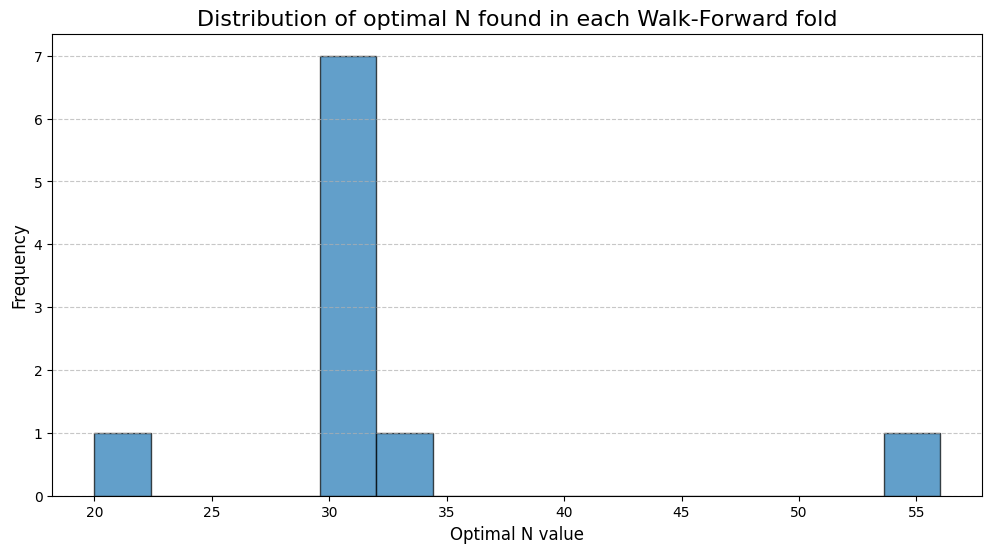
The histogram clearly reveals a bimodal distribution. There are two distinct clusters of optimal N values: one centered around a lower value (~43) and another around a higher value (~58). This is strong evidence of at least two different market regimes being present in our historical data. One regime rewarded a more reactive model (lower N), while the other favored a more deliberate, trend-following approach (higher N).
A simple average (~50) would yield a compromise parameter that was not actually optimal during any of the identified regimes. This necessitates a more sophisticated method for our final parameter selection. We must algorithmically identify these clusters and then determine which cluster corresponds to a more stable and profitable trading regime.
Advantages of this variant (WFCV):
Unlike k-fold CV in machine learning, WFCV does not shuffle data. Each training set precedes the test set in time, avoiding lookahead bias.
By re-estimating parameters on rolling or expanding windows, the model continuously adapts to new data regimes.
It mirrors how a strategy would have been updated in production: fit on past, tested on future.
Performance is measured across multiple test windows. This avoids over-optimism that comes from testing on just one period.
If performance degrades across successive folds, it signals fragility or regime dependence.

K-Means clustering to identify parameter regimes
The task of identifying natural groupings in data is a canonical application for unsupervised machine learning, specifically clustering algorithms. We will employ the K-Means algorithm to analyze the distribution of our best_ns_from_folds.
The objective of K-Means is to partition a set of n data points into k distinct clusters, S=S1,S2,...,Sk. The algorithm aims to minimize the within-cluster sum of squares (WCSS), also known as inertia.
If you want to know more about K-Means and other clustering techniques, don’t forget to check the clustering series:
The within-cluster sum of squares (WCSS), also known as inertia, measures how internally coherent the clusters are. The objective function is defined as:
where:
k is the number of clusters,
Si is the set of data points assigned to cluster i,
x is a data point, and
μi is the centroid (mean) of cluster i.
The algorithm iterates between two main steps:
Assignment step:
Each data point is assigned to the cluster whose centroid is nearest in terms of Euclidean distance:
\(S_i^{(t)} = \left\{ x_p : \|x_p - \mu_i^{(t)}\|^2 \leq \|x_p - \mu_j^{(t)}\|^2 \;\; \forall j, \; 1 \leq j \leq k \right\}\)Update step:
The centroids are updated by recalculating them as the mean of all data points assigned to each cluster:
\(\mu_i^{(t+1)} = \frac{1}{|S_i^{(t)}|} \sum_{x_p \in S_i^{(t)}} x_p\)
A robust implementation requires a smart initialization of the centroids. We use the K-Means++ method, which probabilistically chooses initial centroids that are spread far apart, leading to better and more consistent results.
class KMeansNumpy:
"""
Implementation of the K-Means algorithm from scratch using NumPy.
Includes K-Means++ initialization for greater robustness.
"""
def __init__(self, k, max_iter=300, random_state=None):
self.k = k
self.max_iter = max_iter
self.random_state = random_state
self.cluster_centers_ = None
self.labels_ = None
def _initialize_centroids_kmeans_plusplus(self, X):
"""Initializes centroids using the K-Means++ method."""
if self.random_state:
np.random.seed(self.random_state)
n_samples, _ = X.shape
centroids = np.zeros((self.k, X.shape[1]))
# 1. Choose the first centroid at random
centroids[0] = X[np.random.choice(n_samples)]
# 2. Choose the next k-1 centroids
for i in range(1, self.k):
# Calculate the squared distance of each point to the nearest centroid
dist_sq = np.array([min([np.inner(c-x, c-x) for c in centroids[:i]]) for x in X])
# Choose a new centroid with a probability proportional to the squared distance
probabilities = dist_sq / dist_sq.sum()
cumulative_probabilities = probabilities.cumsum()
r = np.random.rand()
new_centroid_idx = np.searchsorted(cumulative_probabilities, r)
centroids[i] = X[new_centroid_idx]
return centroids
def fit(self, X):
"""
Fits the K-Means model to the data X.
"""
self.cluster_centers_ = self._initialize_centroids_kmeans_plusplus(X)
for _ in range(self.max_iter):
# Assignment step: assign each point to the nearest centroid
self.labels_ = np.array([np.argmin([np.linalg.norm(x-c) for c in self.cluster_centers_]) for x in X])
# Update step: recalculate the centroids
new_centers = np.array([X[self.labels_ == i].mean(axis=0) for i in range(self.k)])
# Check for convergence
if np.allclose(self.cluster_centers_, new_centers):
break
self.cluster_centers_ = new_centers
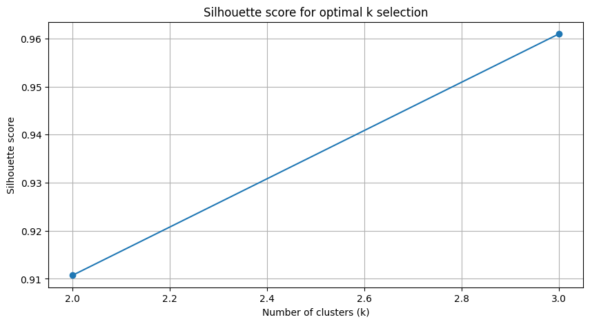
return selfA critical choice in K-Means is the value of k. An objective method is to use the Silhouette Score. This metric evaluates the quality of the clustering by measuring both cluster cohesion and separation. For a single data point i, its Silhouette Score s(i) is:
where a(i) is the mean distance between i and all other points in the same cluster, and b(i) is the mean distance from i to all points in the next nearest cluster. The score ranges from -1 to 1; a higher score indicates better-defined clusters. We can automate the selection of k by iterating through a range of possible values (e.g., 2 to 10) and choosing the one that maximizes the average Silhouette Score across all data points.
Advantage of applying clustering to WFCV
Clustering parameters (hyperparameter space):
After running WFCV with different parameter sets, you’ll often get a cloud of results.
Clustering helps identify stable regions of parameters (robust optima) rather than single lucky configurations.
Avoids overfitting to isolated parameter values by choosing clusters of good solutions.
Clustering market regimes (data segments):
Markets cycle through regimes (trending, mean-reverting, volatile, calm).
Clustering historical periods by features (volatility, correlation, liquidity) allows you to:
Apply WFCV separately by regime.
Assess how the strategy performs under different market conditions.
Potentially select parameters conditioned on regime.
Clustering performance profiles:
If you track multiple metrics across walk-forward folds (e.g., Sharpe, drawdown, skew), clustering can group “consistent” folds together.
This identifies structural consistency versus noise-driven wins.
Why combine them?
WFCV alone tells you how robust a model is across time.
Clustering on top of WFCV tells you whether there are patterns in that robustness—for example, a strategy only works in high-volatility regimes, or only for a band of parameter values.
Together, they give a double filter against overfitting:
Temporal validation (WF).
Structural validation (clustering of parameters/regimes).
This helps you move toward structurally robust strategy.
Final selection of parameters
We have now reached the final synthesis. We possess the distribution of historically optimal parameters from our WF and the K-Means algorithm to analyze it. The final procedure is as follows:
Find optimal k: Apply the
find_optimal_kfunction to thebest_ns_from_foldsdata to determine the number of distinct parameter regimes.Run K-Means: Train the K-Means algorithm using the optimal k. This partitions the historically best N values into distinct clusters.
Evaluate cluster performance: This is the critical step that links clustering back to profitability. For each identified cluster, we calculate the average out-of-sample
test_metricof all the WF folds whose optimal N belongs to that cluster.Select winning cluster: We identify the cluster that exhibits the highest average out-of-sample performance. This represents the most robust and historically profitable parameter regime.
Determine final parameter: Our final, robust parameter N for live deployment is the centroid of this winning cluster, rounded to the nearest integer.
This function encapsulates the entire final selection logic.
def find_robust_n_kmeans_auto(results):
    """
    Finds the robust N using K-Means, automating the choice of 'k'
    and selecting the N from the best-performing cluster.
    """
    if not results:
        raise ValueError("The results list is empty.")
    best_ns_in_folds = np.array([res['best_N_in_fold'] for res in results])
    test_metrics = np.array([res['test_metric'] for res in results])
    X = best_ns_in_folds.reshape(-1, 1)

    optimal_k, k_scores = find_optimal_k(X)
    print(f"Searching for k: Optimal k found = {optimal_k} (based on Silhouette Score).")
    if isinstance(k_scores, dict):
        print("Scores for k:", {k: round(s, 3) for k, s in k_scores.items()})

    if optimal_k <= 1:
        print("No significant cluster structure found. Using median as a fallback.")
        return int(np.round(np.median(best_ns_in_folds)))

    kmeans = KMeansNumpy(k=optimal_k, random_state=42).fit(X)
    labels = kmeans.labels_
    centroids = kmeans.cluster_centers_.flatten()

    avg_performance_per_cluster = [np.mean(test_metrics[labels == i]) if len(test_metrics[labels == i]) > 0 else -np.inf for i in range(optimal_k)]
    best_cluster_index = np.argmax(avg_performance_per_cluster)
    robust_n = int(np.round(centroids[best_cluster_index]))

    print(f"Winning Cluster: #{best_cluster_index+1} with centroid N = {robust_n} and avg OOS performance = {avg_performance_per_cluster[best_cluster_index]:.3f}")
    return robust_n
The entire process—WF optimization, clustering, and centroid selection—has been conducted on a validation dataset (e.g., the first 50% of our total data). The ultimate test of the methodology is to apply the selected robust parameter N to a completely untouched hold-out set (the final 50%). This provides the least biased estimate of future performance.
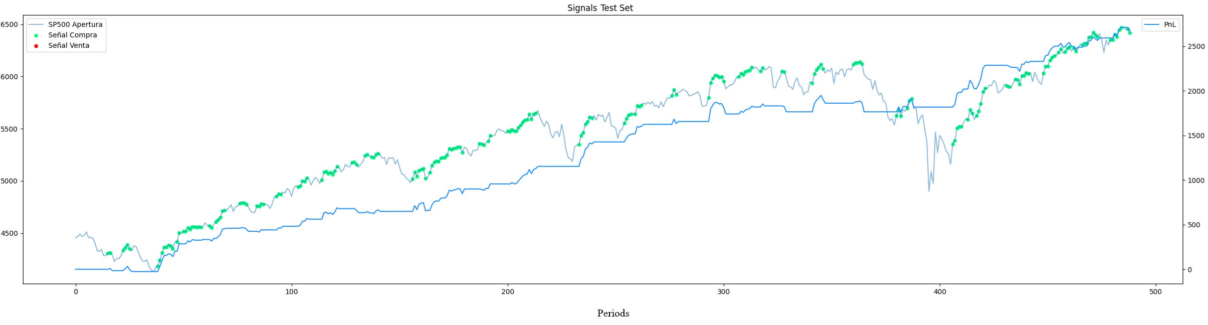
This final chart is the culmination of our process. It does not depict the idealized, overfitted curve of a naive optimization. Instead, it presents a realistic performance profile, in two years OOS—the PnL is the blue line. Critically, this performance was achieved on entirely unseen data, using a single parameter selected through a methodology explicitly designed to prioritize stability and out-of-sample robustness over fragile, in-sample perfection.
The performance of this inefficiency alone was already acceptable, but now it has been fine-tuned.
This process is not an oracle; no methodology in quantitative finance is. The future can, and will, introduce dynamics unseen in the past. However, this framework replaces the speculative hope of a perfect backtest with a rigorous, scientifically-grounded procedure. It is a frank acknowledgment that while we cannot predict the future, we can construct systems engineered to be resilient to its inherent uncertainty.

Time to reset your models and recharge guys! Keep backtesting, keep optimizing, keep that alpha-hunting spirit sharp! Stay quanty!📈
PS: How often do you optimize your models?
Appendix
Full method
import numpy as np

def propagate_ones(input_array, N):
    result = np.array(input_array)
    for _ in range(N):
        shifted = np.roll(result, -1)
        can_propagate = (result == 1) & (shifted == 0)
        result[np.where(np.roll(can_propagate, 1))] = 1
    return result

def propagate_minus_ones(input_array, N):
    result = np.array(input_array)
    for _ in range(N):
        shifted = np.roll(result, -1)
        can_propagate = (result == -1) & (shifted == 0)
        result[np.where(np.roll(can_propagate, 1))] = -1
    return result


def robust_normalization(data):
    valid_data = data[~np.isnan(data) & ~np.isinf(data)]
    if valid_data.size == 0:
        return np.zeros_like(data)
    q80, q20 = np.quantile(valid_data, [0.8, 0.2])
    if q80 == q20:
        return np.zeros_like(data)
    return (data - q80) / (q80 - q20)

# 1. K-MEANS IMPLEMENTATION AND ITS COMPONENTS FROM SCRATCH
class KMeansNumpy:
    """
    Implementation of the K-Means algorithm from scratch using NumPy.
    Includes K-Means++ initialization for greater robustness.
    """
    def __init__(self, k, max_iter=300, random_state=None):
        self.k = k
        self.max_iter = max_iter
        self.random_state = random_state
        self.cluster_centers_ = None
        self.labels_ = None

    def _initialize_centroids_kmeans_plusplus(self, X):
        """Initializes centroids using the K-Means++ method."""
        if self.random_state:
            np.random.seed(self.random_state)

        n_samples, _ = X.shape
        centroids = np.zeros((self.k, X.shape[1]))

        # 1. Choose the first centroid at random
        centroids[0] = X[np.random.choice(n_samples)]

        # 2. Choose the next k-1 centroids
        for i in range(1, self.k):
            # Calculate the squared distance of each point to the nearest centroid
            dist_sq = np.array([min([np.inner(c-x, c-x) for c in centroids[:i]]) for x in X])

            # Choose a new centroid with a probability proportional to the squared distance
            probabilities = dist_sq / dist_sq.sum()
            cumulative_probabilities = probabilities.cumsum()
            r = np.random.rand()

            new_centroid_idx = np.searchsorted(cumulative_probabilities, r)
            centroids[i] = X[new_centroid_idx]

        return centroids

    def fit(self, X):
        """
        Fits the K-Means model to the data X.
        """
        self.cluster_centers_ = self._initialize_centroids_kmeans_plusplus(X)

        for _ in range(self.max_iter):
            # Assignment step: assign each point to the nearest centroid
            self.labels_ = np.array([np.argmin([np.linalg.norm(x-c) for c in self.cluster_centers_]) for x in X])

            # Update step: recalculate the centroids
            new_centers = np.array([X[self.labels_ == i].mean(axis=0) for i in range(self.k)])

            # Check for convergence
            if np.allclose(self.cluster_centers_, new_centers):
                break

            self.cluster_centers_ = new_centers

        return self

def silhouette_score_numpy(X, labels):
    """
    Calculates the Silhouette Score from scratch. It measures how well the points are clustered.
    A higher value indicates denser and better-separated clusters.
    """
    n_samples = len(X)
    unique_labels = np.unique(labels)
    n_clusters = len(unique_labels)

    if n_clusters < 2:
        return 0  # Cannot be defined for a single cluster

    # Calculate the mean intra-cluster distance (a) for each point
    a = np.zeros(n_samples)
    for i in range(n_clusters):
        cluster_mask = (labels == i)
        cluster_points = X[cluster_mask]
        if len(cluster_points) > 1:
            # Distance of each point to all others in its cluster
            dists = np.linalg.norm(cluster_points[:, np.newaxis] - cluster_points, axis=2)
            a[cluster_mask] = np.sum(dists, axis=1) / (len(cluster_points) - 1)

    # Calculate the mean distance to the nearest cluster (b) for each point
    b = np.zeros(n_samples)
    for i in range(n_clusters):
        cluster_mask = (labels == i)
        # Mean distance to all other clusters
        other_cluster_dists = np.array([
            np.mean(np.linalg.norm(X[cluster_mask] - c, axis=1)) for c in np.unique(X[labels != i], axis=0)
        ])
        if len(other_cluster_dists) > 0:
            b[cluster_mask] = np.min(other_cluster_dists)
        else: # In case there is only one cluster with points
            b[cluster_mask] = 0

    # Calculate the Silhouette score for each point and then average
    # s = (b - a) / max(a, b)
    with np.errstate(divide='ignore', invalid='ignore'):
        s = (b - a) / np.maximum(a, b)
    s[np.isnan(s)] = 0 # Cases where a and b are 0

    return np.mean(s)


def find_optimal_k(X, max_k=10):
    """
    Automates the search for the optimal number of clusters 'k'
    by finding the one that maximizes the Silhouette Score.
    """
    if len(np.unique(X)) < 2:
        return 1, -1 # Cannot cluster if all points are the same

    # The maximum number of clusters cannot be greater than the number of samples - 1
    k_range = range(2, min(max_k, len(np.unique(X))))
    if not k_range:
        return 1, -1

    scores = {}
    for k in k_range:
        kmeans = KMeansNumpy(k=k, random_state=42).fit(X)
        score = silhouette_score_numpy(X, kmeans.labels_)
        scores[k] = score

    if not scores:
        return 1, -1

    # The optimal k is the one with the highest Silhouette Score
    optimal_k = max(scores, key=scores.get)
    return optimal_k, scores

# 2. TimeSeriesSplitNumpy and Helper Functions (No changes)
class TimeSeriesSplitNumpy:
    def __init__(self, n_splits=5, max_train_size=None, embargo_size=0):
        self.n_splits, self.max_train_size, self.embargo_size = n_splits, max_train_size, embargo_size
    def split(self, data):
        n_samples = len(data)
        indices = np.arange(n_samples)
        n_test_samples = n_samples // (self.n_splits + 1)
        start_test_index = n_samples - self.n_splits * n_test_samples
        for _ in range(self.n_splits):
            train_end_index = start_test_index - 1 - self.embargo_size
            if train_end_index < 0: continue
            train_indices = indices[:train_end_index + 1]
            test_indices = indices[start_test_index : start_test_index + n_test_samples]
            if self.max_train_size and len(train_indices) > self.max_train_size:
                train_indices = train_indices[-self.max_train_size:]
            yield train_indices, test_indices
            start_test_index += n_test_samples

def backtesting(price, signals, commissions, shift=1):
    price, signals = np.array(price), np.array(signals)
    signals_shifted = np.roll(signals, shift); signals_shifted[:shift] = 0
    price_diff = np.diff(price, prepend=price[0])
    returns = signals_shifted[1:] * price_diff[1:]
    trades = np.diff(signals_shifted, prepend=0)
    costs = np.abs(trades[1:]) * commissions
    return np.cumsum(returns - costs)


# 3. MAIN CV FUNCTION WITH AUTOMATED K-MEANS
def find_robust_n_kmeans_auto(results):
    """
    Finds the robust N using K-Means, automating the choice of 'k'
    and selecting the N from the best-performing cluster.
    """
    if not results:
        raise ValueError("The results list is empty.")

    best_ns_in_folds = np.array([res['best_N_in_fold'] for res in results])
    test_metrics = np.array([res['test_metric'] for res in results])

    # K-Means needs a 2D array
    X = best_ns_in_folds.reshape(-1, 1)

    # 1. Automate the search for the optimal 'k'
    optimal_k, k_scores = find_optimal_k(X)
    print(f"Searching for k: Optimal k found = {optimal_k} (based on Silhouette Score).")
    # Check if k_scores is a dictionary before trying to print it.
    if isinstance(k_scores, dict):
        print("k scores:", {k: round(s, 3) for k, s in k_scores.items()})
    # If k=1, it means there is no cluster structure, so we use the median
    if optimal_k == 1:
        print("No cluster structure found. Using the median as a fallback.")
        return int(np.round(np.median(best_ns_in_folds)))

    # 2. Train K-Means with the optimal k
    kmeans = KMeansNumpy(k=optimal_k, random_state=42).fit(X)
    labels = kmeans.labels_
    centroids = kmeans.cluster_centers_.flatten()

    # 3. Select the N from the most profitable cluster
    avg_performance_per_cluster = []
    for i in range(optimal_k):
        metrics_in_cluster = test_metrics[labels == i]
        avg_performance_per_cluster.append(np.mean(metrics_in_cluster) if len(metrics_in_cluster) > 0 else -np.inf)

    best_cluster_index = np.argmax(avg_performance_per_cluster)
    robust_n = int(np.round(centroids[best_cluster_index]))

    print(f"Winning cluster: {best_cluster_index+1} with average N = {robust_n} and OOS performance = {avg_performance_per_cluster[best_cluster_index]:.3f}")

    return robust_n

def robust_walk_forward_cv_kmeans(price, data_series, model_function, k_folds=5, N_range=(40, 60), step=2, embargo_size=0):
    """
    Performs Walk-Forward CV and then uses automated K-Means to choose the final N.
    """
    results = []
    tscv = TimeSeriesSplitNumpy(n_splits=k_folds, embargo_size=embargo_size)

    # The PnL and cosine similarity are used as the fitness metric in training
    # to choose the best N in each fold
    def get_fitness_score(pnl, price):
        if len(pnl) < 2: return -np.inf
        # Example: Sharpe Ratio (simplified, assuming risk-free rate = 0)
        returns = np.diff(pnl, prepend=0)
        sharpe = np.mean(returns) / (np.std(returns) + 1e-9)
        return sharpe

    for fold_num, (train_indices, test_indices) in enumerate(tscv.split(data_series)):
        print(f"Processing fold {fold_num + 1}/{k_folds}...")
        if not len(train_indices) or not len(test_indices): continue

        train_data, train_price = data_series[train_indices], price[train_indices]
        test_data, test_price = data_series[test_indices], price[test_indices]
        if len(train_data) < N_range[0]: continue

        best_metric_train, best_N = -np.inf, None
        for N in range(N_range[0], N_range[1] + 1, step):
            if len(train_data) < N: continue
            signals = model_function(train_data, N)
            pnl = backtesting(train_price, signals, commissions=0)
            metric = get_fitness_score(pnl, train_price)
            if metric > best_metric_train:
                best_metric_train, best_N = metric, N

        if best_N is None: continue

        signals_test = model_function(test_data, best_N)
        pnl_test = backtesting(test_price, signals_test, commissions=0)
        test_metric = get_fitness_score(pnl_test, test_price)

        results.append({
            "best_N_in_fold": best_N, "test_metric": test_metric
        })

    best_N_robust = find_robust_n_kmeans_auto(results)
    return results, best_N_robust

def model_signal(series, N, signal_propagation=1):
    """
    FILL THIS WITH YOUR MODEL AND THE SIGNALS IT PRODUCES
    """
    # Placeholder for signals, replace with actual model logic
    signals = np.zeros_like(series)
    return signals