


Table of contents:
Introduction.
Risks and limitations.
Foundation of free-parameter optimization.
The foundational problem.
Adaptive gradient methods.
Learning from a stream.
A new perspective on optimization.
Beyond euclidean distance.
Second-order methods.
Beyond convexity.
Before you begin, remember that you have an index with the newsletter content organized by clicking on “Read full story” in this image.

Introduction
Let’s talk plainly. Quant finance has spent years chasing complexity—layering indicators, stacking models, scaling clusters—anything that might tease out an edge. We’ve built whole infrastructures around that chase: faster data, bigger grids, deeper nets. Yet under all that polish sits an awkward truth we rarely lead with: most strategies lean on hand-picked knobs. Call them hyperparameters, call them settings—either way, they’re the quiet choices that end up steering the ship.
You see it everywhere. A moving-average crossover needs window lengths. A mean-reversion rule needs a lookback and a band. A volatility breakout wants a multiplier. Walk into modern ML and the stakes rise: learning rate, weight decay, batch size, scheduler. Even outside modeling, our pipeline is studded with dials—rebalancing frequency, slippage assumptions, position caps. We burn weeks on sweeps and cross-validation, convinced that if we just explore the space thoroughly enough we’ll pin down the magic combination. The graphs look great. The write-ups are neat. Then the market shifts—and the optimal setting turns into a liability we didn’t budget for.
That’s the heart of the problem. Tuning works only if the distribution you tuned on sticks around. Markets don’t make that promise. Correlations flip. Liquidity thins and floods. Volatility breathes. Sometimes, the world simply changes. The parameters we crowned on last quarter’s tape are calibrated to conditions that have already moved on. It’s not that the idea is broken; it’s that our chosen settings are brittle. We’re trading our hyperparameters as much as we’re trading our thesis, and hyperparameters don’t age well.
Optimization is supposed to be the bridge between insight and execution. Too often it becomes a craft project. We define the model, expose the levers, and then babysit them—choosing search ranges, deciding early-stopping rules, picking which metric to maximize, picking which metric to trust when the others disagree. Even when the search is automated, the meta-choices are ours. That’s human judgment sneaking in the side door and, with it, human bias. If the goal is to automate discovery and deployment, it’s odd that our process still hinges on manual nudges at the most sensitive steps.
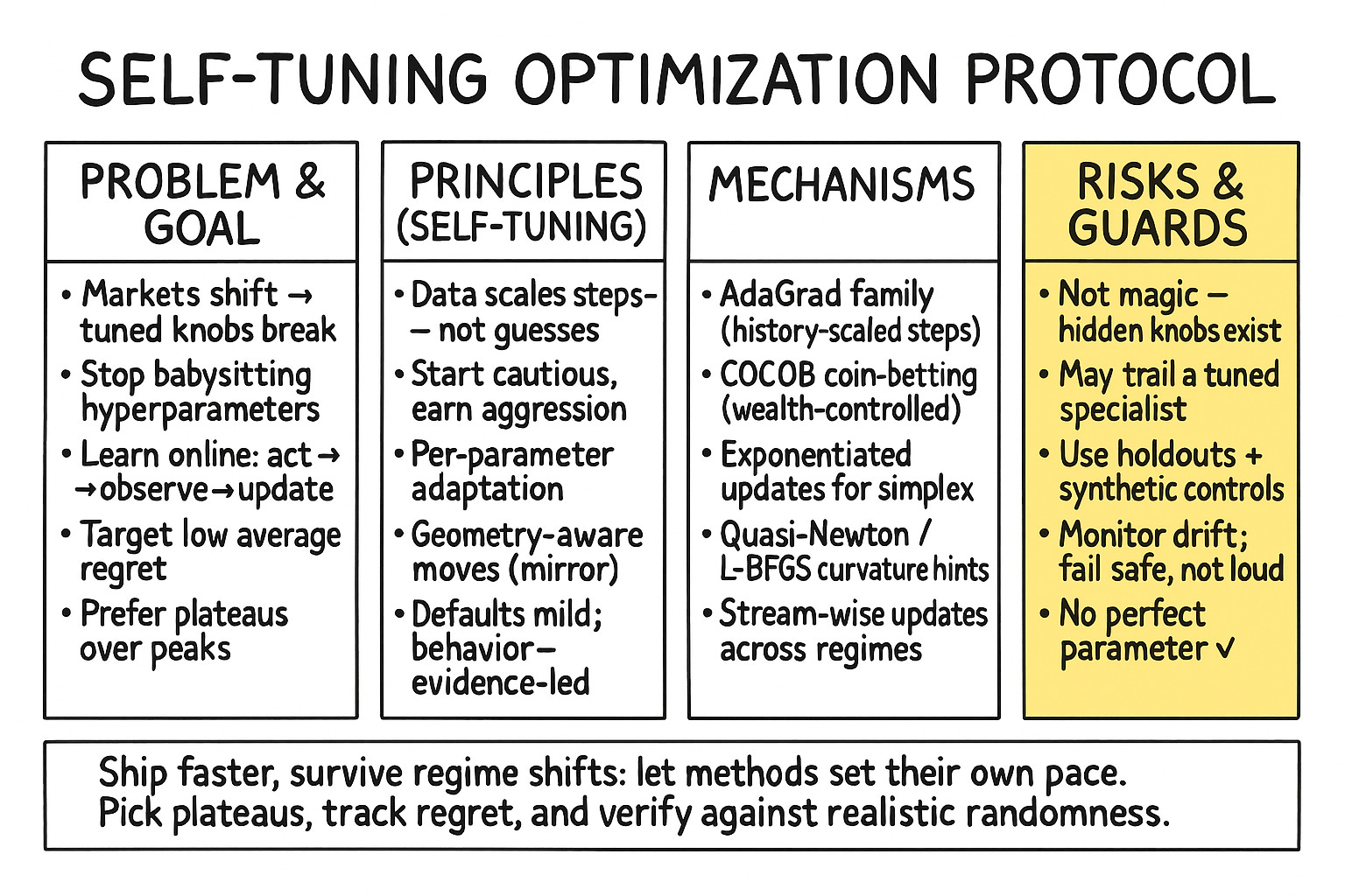
There’s a cleaner path: methods that set their own pace. Think of algorithms that scale steps by what the data actually delivers—by the observed magnitude and variability of gradients, by how reliably a step reduces loss, by whether a local model’s promises match reality. Instead of asking you for a learning rate, they infer one implicitly. Instead of committing to a fixed step, they back off when progress disappoints and press when the path is clear. Instead of assuming the data’s scale and smoothness, they measure it as they go and adapt on the fly.
Call that parameter-free if you like; “self-tuning” might be the more honest label. If you want to know a little bit more, check this presentation:
The appeal isn’t that all choices disappear. It’s that the sensitive ones—the dials that traditionally make or break a run—are absorbed into rules that react to the stream. That shift pays off in three practical ways. First, time-to-first-trade drops. You spend less energy hunting an initial learning rate or momentum combo that won’t explode. Second, robustness rises. When volatility doubles or signal strength fades, the method adjusts its stride without a full retrain cycle. Third, collaboration gets easier. New ideas move to live faster because the brittle, black-art phase shrinks.
Sadly, “parameter-free” isn’t “parameter-less”—think about that, if it’s really parameter-free, then there is no need for optimization. Guardrails exist. Safeguards exist. Defaults exist. But the defaults are mild and the method’s behavior is dominated by what the data reveals—not by what we guessed in advance. That’s exactly where we want the weight of decision-making in a domain where the tape keeps rewriting itself.
Risks and limitations
Now, before we declare the death of parameter tuning and pop the champagne, let’s address the risks. The very term parameter-free can sound like snake oil. Is anything truly free of parameters, or are they just hidden under a more complex layer of abstraction? This is a valid concern. Early adaptive methods, for instance, often introduced new, even more esoteric parameters to tune.
The primary risk is performance. Can an algorithm that has to learn everything from scratch, including its own learning rate, compete with a finely-tuned, specialized model? The fear is that in trying to be a jack-of-all-trades, it becomes a master of none. It might adapt, but too slowly to capture fleeting alpha, resulting in a consistent, but mediocre, performance.
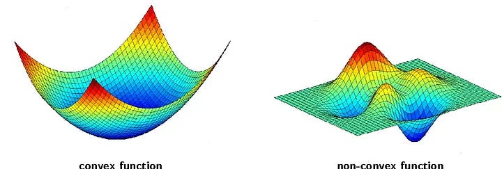
Another significant risk lies in the theoretical underpinnings. The guarantees for many optimization algorithms rely on assumptions that are, to put it mildly, heroic in a financial context. The most common is the assumption of convexity in the loss function. While we can often frame our problems to be convex (e.g., minimizing tracking error), the true profit-and-loss surface of any real-world strategy is a monstrous, non-convex beast. How does a parameter-free algorithm behave when its foundational assumptions are violated? Does it fail gracefully or does it blow up spectacularly?
The core conflict that drives the need for this new approach is the fundamental mismatch between our tools and our environment. We are using static optimization techniques, which implicitly assume a stable world, to trade financial markets, one of the most dynamic and adversarial systems ever created by humankind.
The pivotal event, repeated daily in trading firms across the globe, is the failure of a once-great model. A quant develops a strategy, tunes it to perfection on five years of data, and it works brilliantly for six months. Then, a central bank makes an unexpected announcement, a new technology disrupts an industry, or a geopolitical crisis unfolds. The market’s statistical properties shift. The model’s performance degrades. The quant is then faced with a choice: go back to the drawing board and re-tune everything, hoping to catch up to the new reality, or watch the strategy slowly die.
This cycle of manual re-tuning is a losing battle. It’s reactive, not proactive. It’s a race we can’t win. The only way to break the cycle is to build algorithms that tune themselves. This is the central challenge: to create optimizers that can autonomously adapt their behavior in response to the stream of data the market provides, without a human in the loop frantically twisting dials. One of the potential solution to this conflict lies in parameter-free optimization.

Foundation of free-parameter optimization
The foundation rests on three main pillars:
The shift from a static to a dynamic marketview (online learning).
The concept of regret.
Elegant adaptive mechanisms that replace manual tuning.
Let’s dissect each one.
The single most important foundational concept is the rejection of the traditional batch learning model.

In the old paradigm, you’d collect a massive, static dataset (say, five years of market data). You’d then split it, tune your hyperparameters (like the learning rate) via a painful process like grid search, train your model, and then deploy it. The problem? The model is instantly a fossil. It’s an expert on the past, but the market has already moved on.
Parameter-free optimization is built on the Online Learning framework. The world is not a static dataset; it’s a continuous, potentially adversarial, stream of data. The process looks like this, repeated indefinitely:
At time
t, the algorithm makes a prediction or takes an action (e.g., sets its portfolio of strategies).The market reveals the outcome.
The algorithm suffers a loss based on the quality of its action.
The algorithm uses this new information (specifically, the gradient of the loss) to update itself and prepare for time
t+1.
This is the natural cadence of financial markets. This shift from a static to a dynamic, iterative process is the absolute bedrock. It forces us to think about algorithms that learn incrementally and continuously.
So, if the market is a continuous stream, how do we even measure performance? We can’t use a fixed test set. The foundational metric here is regret.
In simple terms, regret is the difference between your algorithm’s total cumulative loss over T time steps and the total loss of the single best, fixed strategy you could have chosen in hindsight.
Let’s formalize it slightly. If your algorithm chose parameters wt at each step, and the best single fixed parameter vector over the whole period was w*, the regret RT is:
The goal of a good online algorithm is to have sublinear regret. This means that the average regret, Rt/T, goes to zero as time goes on. Anyone would say this is a guarantee that your algorithm will work as if it knew the entire future in advance and picked the best single set of parameters. But nothing could be further from the truth: if you don’t structure it well, the losses can be monumental.
Then, how do we build algorithms that can achieve this low regret without a learning rate? This is where the clever mechanisms come in. They all revolve around one idea: Use the history of the data stream to inform future actions.
Two foundational approaches stand out:
Adaptive subgradient methods (the AdaGrad family): This was the first major breakthrough. The intuition is simple but key. Instead of one learning rate for all parameters, let’s have one for each. And let’s scale that learning rate based on what we’ve seen. The core idea is to accumulate the sum of the squares of the gradients for each parameter. The update for a parameter wi looks something like:
\(\Delta w_i \;=\; -\,\frac{\eta}{\sqrt{\sum g_i^{2}}}\, g_i\)This means parameters that have received large, frequent gradient updates in the past (high sum of squares) will have their effective learning rate shrink. Infrequent parameters will see larger updates. The algorithm learns the geometry of the problem and adapts its step sizes accordingly, effectively creating its own learning rate schedule on the fly.
AdaGrad family Coin-betting algorithms (the COCOB family): This is a more recent and, arguably, more elegant foundation. It reframes the entire optimization problem as a betting game. At each step, the algorithm “bets” some of its internal “wealth” on the direction of the gradient.
If the bet is correct (the update reduces the loss), its wealth increases.
If the bet is wrong, its wealth decreases. The size of the next parameter update is directly proportional to this wealth. A wealthy, confident algorithm takes large steps. A poor, uncertain algorithm takes tiny, cautious steps. The learning rate is completely replaced by this internal, self-regulating state of wealth. It’s a beautiful, parameter-free mechanism for controlling the optimization process.

COBOT family

This foundation is pretty cool because it takes into account:
The dynamic view of the market (online learning).
A suitable performance metric (regret—but could be any other metric).
Self-tuning mechanism (adaptive history or coin-betting—In future publications we will see other more specific algorithms for this.)
The foundational problem
The learning rate is, without a doubt, the most critical hyperparameter in the vast majority of optimization algorithms used in machine learning and, by extension, in quantitative trading. It is the knob that controls the step size of the optimization process, the dial that determines how aggressively the algorithm updates its parameters in response to new information. Get it right, and you have a model that learns efficiently and converges to a good solution. Get it wrong, and you have a model that either learns at a glacial pace or, worse, overshoots the optimal solution and diverges into instability. This is the tyranny of the learning rate: a single, seemingly innocuous parameter that holds the fate of your model in its hands.
Let’s make this more concrete with a bit of mathematics. Consider the canonical stochastic gradient descent algorithm, the workhorse of modern machine learning. The update rule for the model parameters, denoted by the vector w, is given by:
Here, wt is the parameter vector at time step t, ηt is the learning rate, and ∇L(wt;xt,yt) is the gradient of the loss function L with respect to the parameters, evaluated at the current parameter vector and a single data point (xt, yt). The choice of ηt is critical. If it is too small, the parameter updates will be minuscule, and the algorithm will take an inordinate amount of time to converge. If it is too large, the updates will be too aggressive, and the algorithm may overshoot the minimum of the loss function, oscillating wildly or even diverging completely.
The traditional approach to this problem is to use a learning rate schedule, where the learning rate is gradually decreased over time. A common choice is to set ηt=η0/(1+αt) where η0 is the initial learning rate and α is a decay parameter. This is a step in the right direction, but it simply replaces one hyperparameter with two. The choice of η0 and α is still a matter of trial and error, a process that is both time-consuming and computationally expensive.
This is where the idea of a parameter-free approach begins to take shape. What if, instead of specifying a learning rate schedule, we could have an algorithm that automatically adapts the learning rate as it goes? This is the core idea behind a class of algorithms known as adaptive gradient methods, which we will explore in the next section.
Here’s a simple Python snippet to illustrate the sensitivity of SGD to the choice of the learning rate. We’ll use a simple quadratic loss function, L(w)=w2, whose minimum is at w=0.
import numpy as np

def loss_function(w):
    return w**2

def gradient(w):
    return 2*w

def sgd(w_init, learning_rate, n_iterations):
    w_history = [w_init]
    w = w_init
    for _ in range(n_iterations):
        w = w - learning_rate * gradient(w)
        w_history.append(w)
    return w_history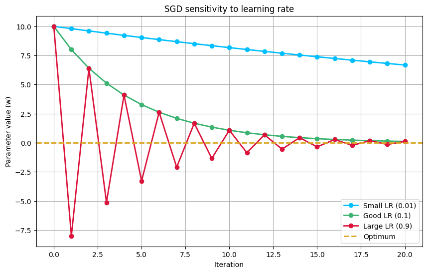
As you can see from the plot, the choice of the learning rate has a dramatic impact on the convergence of the algorithm. The good learning rate converges smoothly and efficiently to the optimal solution. The small learning rate also converges, but at a much slower pace. The large learning rate overshoots the optimum and oscillates around it, failing to converge in the given number of iterations. This simple example highlights the fundamental problem with a fixed learning rate and motivates the need for a more adaptive approach.
Adaptive gradient methods
A new breed of optimization algorithms emerged, armed with the ability to adapt the learning rate for each parameter individually and automatically. These are the adaptive gradient methods, particularly in deep learning where the number of parameters can be too much.
One of the earliest and most influential of these methods is AdaGrad (Adaptive Gradient). The key idea behind AdaGrad is to use a different learning rate for each parameter, and to scale this learning rate based on the history of the gradients for that parameter. The update rule for the i-th parameter at time step t is given by:
Here, η is a global learning rate, gt,i is the gradient of the loss function with respect to the i-th parameter at time step t, and Gt,ii is the sum of the squares of the past gradients for that parameter:
The term ϵ is a small constant added for numerical stability, to prevent division by zero. The intuition behind this update rule is that parameters that have seen large gradients in the past will have their learning rates reduced, while parameters that have seen small gradients will have their learning rates increased. This has the effect of performing larger updates for infrequent parameters and smaller updates for frequent parameters, which is particularly useful for sparse data.
While AdaGrad was a significant step forward, it has a major drawback: the sum of the squared gradients in the denominator is a monotonically increasing quantity. This means that the learning rate is always decreasing, and can eventually become so small that the algorithm stops learning altogether. This is where a subsequent generation of adaptive methods, such as RMSprop and Adam, come into the picture.
RMSprop (Root Mean Square Propagation) addresses the problem of the ever-decreasing learning rate by using a moving average of the squared gradients instead of a sum. The update rule for RMSprop is:
Here, E[g2]t is the moving average of the squared gradients, and γ is a decay parameter that controls the size of the moving average window. This prevents the learning rate from becoming infinitesimally small and allows the algorithm to continue learning even after many iterations.
Adam (Adaptive Moment Estimation) is perhaps the most popular of the adaptive gradient methods. It combines the ideas of RMSprop with the concept of momentum, which helps the algorithm to accelerate in the direction of the gradient and to dampen oscillations. Adam maintains two moving averages: one for the gradients themselves (the first moment) and one for the squared gradients (the second moment). The update rule is a bit more complex, but the core idea is the same: to adapt the learning rate for each parameter based on the history of the gradients.
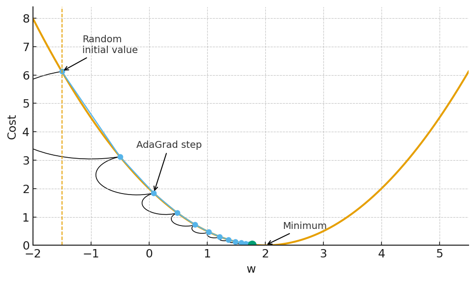
Let’s see how AdaGrad performs on our simple quadratic loss function.
import numpy as np

def loss_function(w):
    return w**2

def gradient(w):
    return 2*w

def adagrad(w_init, learning_rate, n_iterations, epsilon=1e-8):
    w_history = [w_init]
    w = w_init
    G = 0
    for _ in range(n_iterations):
        grad = gradient(w)
        G += grad**2
        w = w - (learning_rate / (np.sqrt(G) + epsilon)) * grad
        w_history.append(w)
    return w_history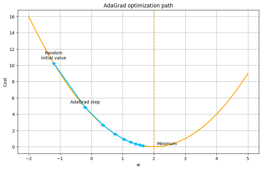
As you can see, AdaGrad converges nicely to the optimal solution. The adaptive nature of the learning rate allows it to make large steps at the beginning when the gradients are large, and smaller steps as it approaches the minimum. This is a significant improvement over the fixed learning rate of SGD. However, these methods are not a panacea. They introduce new hyperparameters of their own (the global learning rate η, the decay parameter γ in RMSprop, and the momentum parameters in Adam). While these are generally less sensitive than the learning rate in SGD, they still require some degree of tuning. The quest for a truly parameter-free algorithm continues.
Learning from a stream
Everybody knows that the market is not static but a continuous stream of information, a firehose of data, news, and order flow. In this environment, the traditional batch learning paradigm, where a model is trained on a fixed dataset, is fundamentally mismatched to the nature of the problem. What is needed is a way to learn from a continuous stream of data, to update our models in real-time as new information becomes available. This is the domain of online learning.
In the online learning framework, the learning process is divided into a sequence of rounds. In each round t, the algorithm makes a prediction, receives the true outcome, and suffers a loss. The goal of the algorithm is to minimize its cumulative loss over time. This is a subtle but important shift from the batch learning setting, where the goal is to minimize the average loss over a fixed dataset.
The connection between online learning and stochastic optimization is a deep one. In fact, any online learning algorithm can be converted into a stochastic optimization algorithm. The key insight is to treat the sequence of loss functions in the online setting as a sequence of stochastic gradients of a single, underlying objective function. This allows us to use the powerful tools and theoretical guarantees of online learning to solve stochastic optimization problems.
One of the most fundamental concepts in online learning is the notion of regret. The regret of an online learning algorithm is the difference between its cumulative loss and the cumulative loss of the best fixed strategy in hindsight. A good online learning algorithm is one that has low regret, meaning that it performs almost as well as if it had known the entire sequence of data in advance.
Let’s formalize this a bit. Let lt(w) be the loss of the algorithm at time step t for a given parameter vector w. The cumulative loss of the algorithm is ∑Tt=1lt(wt), where wt is the parameter vector chosen by the algorithm at time step t. The cumulative loss of the best fixed parameter vector w* in hindsight is ∑Tt=1lt(wt*). The regret is then:
The goal is to design algorithms with sublinear regret, meaning that the average regret, Rt/T, goes to zero as T goes to infinity. This is a powerful guarantee, as it implies that the algorithm is, on average, doing as well as the best fixed strategy.
Many of the adaptive gradient methods we discussed in the previous section, such as AdaGrad, were originally developed in the online learning setting. They have provable regret bounds, which is why they are so effective as stochastic optimization algorithms.
The online learning framework is particularly well-suited to the world of algorithmic trading. A trading strategy can be viewed as an online learning algorithm that is constantly making predictions about the future direction of the market, receiving feedback in the form of profits and losses, and updating its internal model accordingly. The concept of regret has a natural interpretation in this context: it is the difference between the actual profit and loss of the strategy and the profit and loss that could have been achieved with perfect foresight.
Here’s a conceptual Python snippet to illustrate the online learning process in a trading context. We’ll simulate a simple strategy that tries to learn the fair price of an asset.
import numpy as np
import matplotlib.pyplot as plt

# 1) Stream generator (piecewise “fair value”)
def generate_price_stream(seed=7):
    “”“
    Create a non-stationary stream: price_t = v_t + noise_t,
    where v_t is a piecewise-constant ‘fair value’ unknown to the learner.
    “”“
    rng = np.random.default_rng(seed)
    regimes = [
        (100.0, 1.5, 400),  # (level, noise_sigma, length)
        (102.0, 2.0, 400),
        (98.0,  2.2, 400),
        (101.0, 1.6, 300),
    ]
    true_v, y = [], []
    for mu, sig, L in regimes:
        true_v.append(np.full(L, mu))
        y.append(mu + rng.normal(0.0, sig, size=L))
    true_v = np.concatenate(true_v)
    y = np.concatenate(y)
    return y, true_v  # observed price, latent fair value (for visualization)

# 2) Online learner (AdaGrad on squared loss)
class OnlineAdaGrad:
    “”“
    Minimizes l_t(w) = 0.5 * (w - y_t)^2 with online gradient steps.
    - prediction at step t is w_t
    - gradient: (w_t - y_t)
    - update: w_{t+1} = w_t - eta_t * (w_t - y_t)
      with eta_t = lr / (sqrt(G_t) + eps), G_t = sum_{i<=t} grad_i^2
    “”“
    def __init__(self, w0: float, lr: float = 1.0, eps: float = 1e-8):
        self.w = float(w0)
        self.lr = float(lr)
        self.eps = float(eps)
        self.G = 0.0

    def step(self, y_t: float):
        pred = self.w
        grad = (self.w - y_t)
        loss = 0.5 * grad * grad
        self.G += grad * grad
        eta_t = self.lr / (np.sqrt(self.G) + self.eps)
        self.w = self.w - eta_t * grad
        return pred, loss, eta_t

# 3) Regret utilities
def best_fixed_hindsight_loss(y: np.ndarray):
    “”“
    For squared loss with constant parameter w, the best fixed w* in hindsight
    is the mean of all y_t. Return (w*, cumulative loss at w*).
    “”“
    w_star = float(np.mean(y))
    cum_loss_star = 0.5 * np.sum((w_star - y) ** 2)
    return w_star, cum_loss_star

# 4) Demo
def run_demo(plot=True):
    y, v = generate_price_stream(seed=7)
    T = len(y)

    # Initialize learner with the first observation as a naive prior
    learner = OnlineAdaGrad(w0=y[0], lr=1.0, eps=1e-8)

    preds = np.empty(T)
    losses = np.empty(T)
    etas  = np.empty(T)

    for t in range(T):
        preds[t], losses[t], etas[t] = learner.step(y[t])

    # Hindsight comparator
    w_star, loss_star = best_fixed_hindsight_loss(y)
    cum_loss_algo = float(np.sum(losses))
    regret = cum_loss_algo - loss_star
    avg_regret = regret / T

    # Report
    print(”T =”, T)
    print(f”Best fixed w* (hindsight mean): {w_star:.4f}”)
    print(f”Final online estimate w_T:      {learner.w:.4f}”)
    print(f”Cumulative loss (algorithm):    {cum_loss_algo:.2f}”)
    print(f”Cumulative loss (best fixed):   {loss_star:.2f}”)
    print(f”Regret R_T:                     {regret:.2f}”)
    print(f”Average regret R_T/T:           {avg_regret:.6f}”)

    if plot:
        fig, axs = plt.subplots(3, 1, figsize=(10, 9), sharex=False)

        # Stream vs. predictions
        axs[0].plot(y, lw=1, label=”Observed price $y_t$”)
        axs[0].plot(v, c=’lime’, lw=2, alpha=0.8, label=”Latent fair value $v_t$”)
        axs[0].plot(preds, c=’red’, lw=2, label=”Online estimate $w_t$ (AdaGrad)”)
        axs[0].axhline(w_star, ls=”--”, lw=1.5, label=”Best fixed $w^*$ (mean)”)
        axs[0].set_title(”Online learning from a stream (squared loss)”)
        axs[0].legend(loc=”best”)

        # Per-step loss
        axs[1].plot(losses, lw=1)
        axs[1].set_title(r”Instantaneous loss $\ell_t(w_t)=\frac{1}{2}(w_t-y_t)^2$”)

        axs[1].set_ylabel(”loss”)

        # Average regret over time
        cum_losses = np.cumsum(losses)
        cum_star = np.cumsum((y - w_star) ** 2) * 0.5
        R_t = cum_losses - cum_star
        avg_R_t = R_t / (np.arange(T) + 1)
        axs[2].plot(avg_R_t, lw=1.5)
        axs[2].set_title(”Average regret $R_t/t$ (should trend toward 0)”)
        axs[2].set_xlabel(”t”)
        axs[2].set_ylabel(”avg regret”)

        plt.tight_layout()
        plt.show()

if __name__ == “__main__”:
    run_demo(plot=True)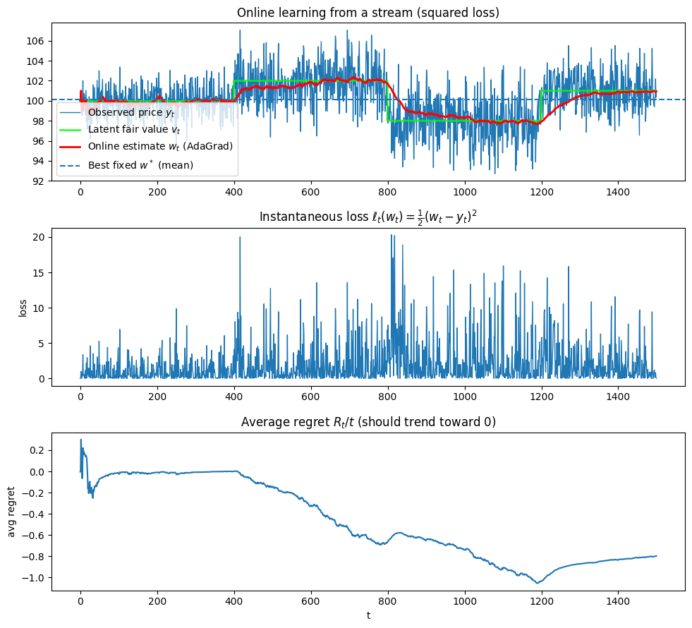
The top panel shows a noisy price stream (blue) with hidden piecewise fair value regimes (green), and the online AdaGrad estimate (red) tracking those regimes: it lags briefly at the change points (around t ≈ 400,800,1150) and then settles, adapting more slowly later because AdaGrad’s effective step size shrinks as gradients accumulate. This simple simulation demonstrates the core principles of online learning.

A new perspective on optimization
The connection between online learning and stochastic optimization is an interesting one, but it is not the only surprising connection that has been uncovered for parameter-free optimization. Another, perhaps even more counter-intuitive, connection is the one between optimization and coin-betting. It turns out that the problem of designing a good optimization algorithm is, in some sense, equivalent to the problem of designing a strategy for betting on a sequence of coin flips, that means, randomly.
This connection was first explored in a seminal paper by Orabona and Pál almost a decade ago, and it has led to a new class of parameter-free optimization algorithms that are both theoretically elegant and practically effective. The core idea is to reframe the optimization process as a game between a player and nature. In each round of the game, nature reveals a gradient, and the player makes a bet on the direction of the next parameter update. The player’s wealth at the end of the game is related to the performance of the optimization algorithm.
Here the paper I mentioned:
Let’s make this more precise. Consider a simple one-dimensional optimization problem where we are trying to find the minimum of a convex function f(w). In each round t, we are given a gradient gt=f′(wt). We can think of the sign of the gradient, sign(gt), as the outcome of a coin flip. If the sign is positive, the minimum is to the left of the current point. If the sign is negative, the minimum is to the right. The problem of choosing the next parameter update is then equivalent to the problem of deciding how much to bet on the outcome of this coin flip.
A good coin-betting strategy is one that can make a profit regardless of the sequence of outcomes, as long as there is some imbalance in the coin. In the context of optimization, this imbalance is provided by the convexity of the function. For a convex function, the gradients will, on average, point towards the minimum. A good coin-betting algorithm can exploit this statistical regularity to make a “profit,” which in this case means moving the parameters closer to the optimal solution.
This connection has led to the development of a number of parameter-free optimization algorithms, such as COCOB (Continuous Coin-Betting) and KT (Kelly-Tuned). These algorithms are able to achieve near-optimal performance without the need for any learning rate tuning. They are able to adapt to the geometry of the loss function and the scale of the gradients automatically, a feat that is difficult to achieve with traditional methods.
The mathematics behind these coin-betting algorithms is quite involved, drawing on ideas from information theory and game theory. However, the intuition is relatively simple. A good betting strategy is to be conservative at the beginning, when you have little information about the coin, and to become more aggressive as you gather more evidence about its bias. Similarly, a good coin-betting optimization algorithm is one that makes small, cautious updates at the beginning of the optimization process, and larger, more confident updates as it gets closer to the optimal solution.
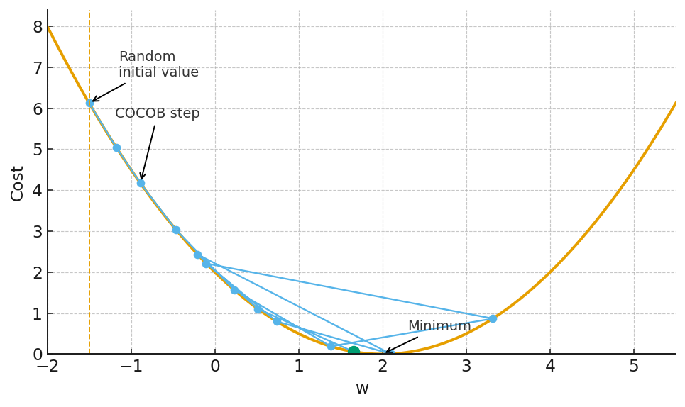
Here is a Python snippet that implements a simplified version of a coin-betting algorithm for our one-dimensional quadratic loss function.
import numpy as np

def loss_function(w):
    return w**2

def gradient(w):
    return 2*w

def coin_betting_optimizer(w_init, n_iterations):
    w_history = [w_init]
    w = w_init
    wealth = 1.0
    for _ in range(n_iterations):
        grad = gradient(w)
        # The “bet” is proportional to the gradient and the current wealth
        bet = grad * wealth * 0.1 # The 0.1 is a constant factor
        w = w - bet
        # The wealth is updated based on the outcome of the “bet”
        wealth = wealth - bet * grad
        w_history.append(w)
    return w_history
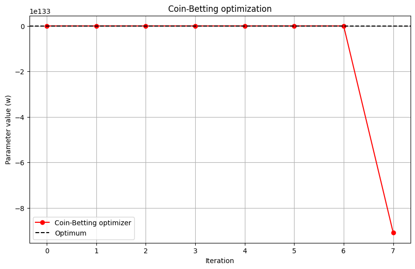
This is a highly simplified implementation, but it captures the essence of the coin-betting approach. The step size of the algorithm is not determined by a pre-specified learning rate, but rather by the internal wealth of the algorithm. This wealth is updated based on the performance of the algorithm, creating a self-tuning mechanism that automatically adapts the learning rate to the problem at hand.
Beyond euclidean distance
The optimization algorithms we have discussed so far, from SGD to adaptive and coin-betting methods, all share a common, implicit assumption: they all operate in a Euclidean space. The parameter updates are all based on the idea of moving in the direction of the negative gradient, and the distance between two parameter vectors is measured by the standard Euclidean distance. This is a natural and intuitive assumption, but it is not always the most appropriate one.
The geometry of the loss function can be highly non-Euclidean. The loss surface can be curved and warped in complex ways, and a step that is optimal in one direction may be far from optimal in another. This is where the idea of mirror descent comes into play. Mirror descent is a generalization of gradient descent that allows us to work in non-Euclidean geometries. The key idea is to use a mirror map to transform the problem from the original, “primal” space into a “dual” space where the geometry is simpler. The gradient descent update is then performed in this dual space, and the result is mapped back to the primal space.
Let’s make this a bit more concrete. In standard gradient descent, the update rule can be seen as the solution to the following optimization problem:
This is a trade-off between making progress on the loss function (the first term) and not moving too far from the current point (the second term). The distance is measured by the squared Euclidean norm.
In mirror descent, we replace the Euclidean distance with a more general measure of distance, called the Bregman divergence. The Bregman divergence is defined in terms of a strictly convex function ϕ, called the potential function. The Bregman divergence between two points w and w′ is given by:
The update rule for mirror descent is then:
By choosing different potential functions, we can induce different geometries on the parameter space. For example, if we choose ϕ(w)=0.5∥w∥22, the Bregman divergence becomes the squared Euclidean distance, and we recover the standard gradient descent algorithm. If we choose a different potential function, we can get algorithms that are better suited to the geometry of the problem at hand.
One of the most common applications of mirror descent is in problems where the parameters are constrained to live in a certain set, such as the probability simplex. In this case, using the standard Euclidean geometry can lead to updates that take the parameters outside of the feasible set, requiring a projection step to bring them back. By choosing an appropriate potential function, such as the negative entropy, we can design a mirror descent algorithm that automatically respects the constraints of the problem, without the need for an explicit projection step. This is the idea behind the exponentiated gradient algorithm, which is widely used in online learning and game theory.
In the context of algorithmic trading, the geometry of the problem is often dictated by the nature of the portfolio construction process. The portfolio weights, for example, are typically constrained to be non-negative and to sum to one. This is precisely the kind of problem where mirror descent can be an interesting tool. By choosing a potential function that is well-suited to the geometry of the portfolio space, we can design optimization algorithms that are both more efficient and more natural than their Euclidean counterparts.
Let’s compare both of them. Here is a Python snippet that illustrates the difference between Euclidean projection and the update of the exponentiated gradient algorithm for a simple portfolio optimization problem—remember that this is only to illustrate the previous idea, ok? It needs quite a bit of refining before it can be used.
import numpy as np

def project_to_simplex(v):
    n_features = v.shape[0]
    u = np.sort(v)[::-1]
    cssv = np.cumsum(u) - 1
    ind = np.arange(n_features) + 1
    cond = u - cssv / ind > 0
    rho = ind[cond][-1]
    theta = cssv[cond][-1] / float(rho)
    w = np.maximum(v - theta, 0)
    return w

def exponentiated_gradient_update(w, grad, learning_rate):
    w = w * np.exp(-learning_rate * grad)
    w = w / np.sum(w)
    return w

w_init = np.array([0.2, 0.3, 0.5])
grad = np.array([-0.1, 0.2, -0.05])
learning_rate = 1.0

# Euclidean update and projection
w_euclidean = w_init - learning_rate * grad
w_euclidean_projected = project_to_simplex(w_euclidean)

# Exponentiated gradient update
w_eg = exponentiated_gradient_update(w_init, grad, learning_rate)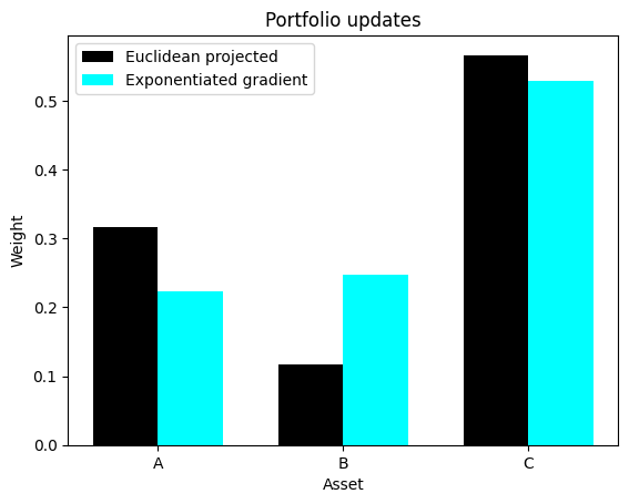
The Euclidean update, followed by a projection, can lead to solutions where some of the weights are set to zero, even if the gradient for that asset is not particularly large. The exponentiated gradient update, on the other hand, produces a smoother and more natural update, where the weights are adjusted multiplicatively. This can be a more desirable behavior in many portfolio optimization problems.
Second-order methods
The optimization methods we have discussed so far are all first-order methods. They rely on the gradient of the loss function to guide the search for the optimal solution. While these methods are simple and often effective, they have a fundamental limitation: they are blind to the curvature of the loss function. They can see the slope of the hill, but they cannot see its shape. This can lead to slow convergence, especially in problems where the loss surface is poorly conditioned, with long, narrow valleys and high-dimensional saddle points.
Second-order methods, as their name suggests, use information from the second derivative of the loss function, the Hessian matrix, to get a more complete picture of the loss surface. The Hessian matrix describes the curvature of the loss function, and it can be used to construct a more direct path to the minimum. The most famous of the second-order methods is Newton’s method. The update rule for Newton’s method is:
Here, Ht is the Hessian matrix of the loss function evaluated at the current parameter vector wt, and [Ht]-1 is its inverse. The term [Ht]-1gt is the Newton step. It can be shown that if the loss function is quadratic, Newton’s method will find the minimum in a single step. For more general functions, it can converge much faster than first-order methods.
However, Newton’s method has a major drawback: the computation of the Hessian matrix and its inverse is computationally expensive. The Hessian matrix has d2 elements, where d is the number of parameters, and inverting it takes O(d3) time. This is prohibitive for high-dimensional problems, such as those encountered in deep learning and many areas of quantitative finance.
This has led to the development of a class of methods known as quasi-Newton methods. These methods try to approximate the inverse of the Hessian matrix using only first-order information. The most famous of these is the Broyden–Fletcher–Goldfarb–Shanno (BFGS) algorithm. The BFGS algorithm maintains an approximation of the inverse Hessian and updates it at each iteration using the change in the parameters and the change in the gradients.
In the context of stochastic optimization, the situation is even more challenging. The Hessian matrix is often not available, and even if it were, it would be a noisy estimate of the true Hessian. This has led to the development of stochastic quasi-Newton methods, which try to approximate the Hessian using noisy gradient information. These methods are an active area of research, and they hold the promise of combining the fast convergence of second-order methods with the scalability of first-order methods.
One of the most successful of these methods is the stochastic L-BFGS algorithm. The “L” stands for “limited-memory,” and it refers to the fact that the algorithm does not store the full approximation of the inverse Hessian, but rather a low-rank approximation based on the last few updates. This makes the algorithm much more memory-efficient and scalable to high-dimensional problems.
Here’s a Python snippet that conceptually illustrates the difference between a first-order and a second-order update on a simple, non-spherical quadratic loss function.
import numpy as np
import matplotlib.pyplot as plt

def loss_function(w):
    return 0.5 * (w[0]**2 + 10 * w[1]**2)

def gradient(w):
    return np.array([w[0], 10 * w[1]])

def hessian(w):
    return np.array([[1, 0], [0, 10]])

w_init = np.array([10, 1])
learning_rate = 0.1

# First-order (SGD) update
w_sgd = w_init - learning_rate * gradient(w_init)

# Second-order (Newton) update
w_newton = w_init - np.linalg.inv(hessian(w_init)) @ gradient(w_init)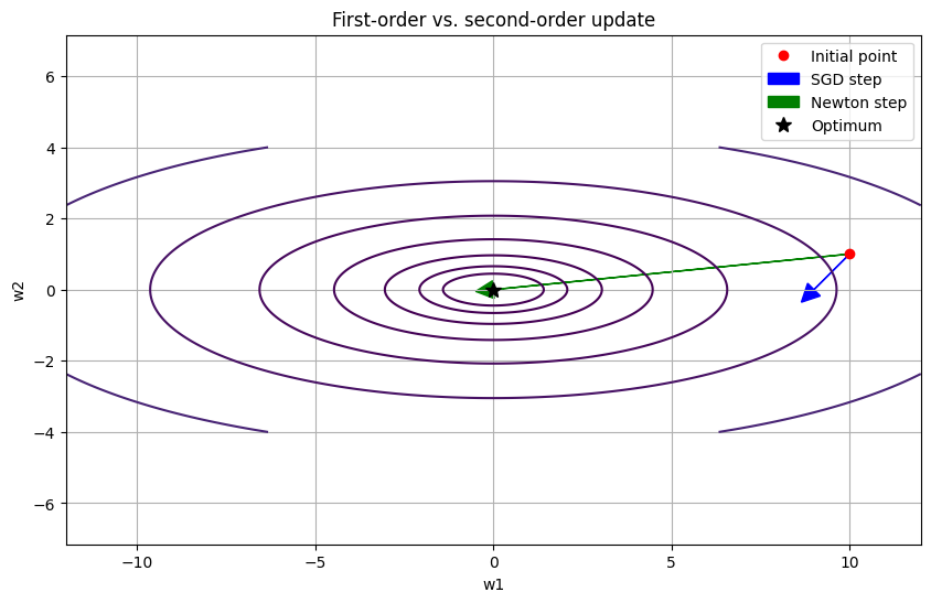
The plot shows the contour lines of a simple quadratic loss function that is elongated in the w2 direction. The SGD step, which is proportional to the negative gradient, does not point directly towards the minimum. It will take many small, zig-zagging steps to reach the bottom of the valley. The Newton step, on the other hand, takes into account the curvature of the loss function and points directly towards the minimum. This is a powerful illustration of the potential benefits of second-order methods.
Beyond convexity
The vast majority of the theoretical results in the field of optimization are for convex functions. Convexity is a powerful property that simplifies the analysis of optimization algorithms and guarantees that any local minimum is also a global minimum. However, the loss functions of many real-world problems, particularly in the realm of deep learning and complex trading strategies, are highly non-convex. They are characterized by a multitude of local minima, saddle points, and flat regions, creating a treacherous landscape for any optimization algorithm.
The challenge of non-convex optimization is one of the most important open problems in the field of machine learning. While there is no single, universally accepted solution, a number of promising research directions have emerged.
One approach is to use techniques from stochastic calculus to analyze the behavior of optimization algorithms in the presence of noise. The addition of noise to the gradient updates, either explicitly or implicitly through the use of stochastic gradients, can help the algorithm to escape from local minima and to explore the loss landscape more effectively. This is the idea behind techniques such as simulated annealing and stochastic gradient Langevin dynamics.
Another approach is to focus on finding good enough solutions, rather than trying to find the global minimum. In many high-dimensional problems, the difference in performance between different local minima can be small. The goal, then, is not to find the single best solution, but rather to find a solution that generalizes well to unseen data. This has led to a renewed interest in the geometry of the loss function and the relationship between the flatness of a minimum and its generalization performance.
In the context of parameter-free optimization, the challenge is to develop algorithms that can navigate the non-convex landscape without the need for manual tuning of parameters such as the learning rate or the amount of noise to add. The coin-betting and adaptive gradient methods we have discussed have shown some promise in this regard, but their theoretical guarantees are often weaker in the non-convex setting.

Nice work today, team! 💪🏻 Now hit refresh on those models and recharge your brains. Let’s stay sharp, stay systematic, and stay quanty! 📊
PS: Do you prefer to find a true positive inefficiency or to rotate spurious strategies?
This is an invitation-only access to our QUANT COMMUNITY, so we verify numbers to avoid spammers and scammers. Feel free to join or decline at any time. Tap the WhatsApp icon below to join
