[WITH CODE] Options: Iron Butterfly

Strategies with options Part II

---

Table of contents:

1. Introduction.

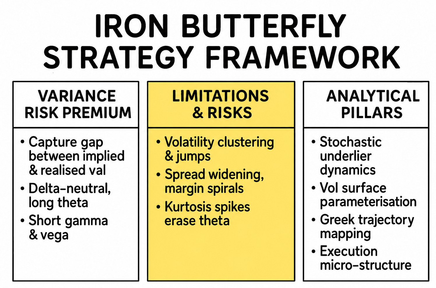
2. Variance risk premium.

3. Limitations and risks.

4. Deconstruction of the analytical framework.

   1. Pillar 0: Structural decomposition into vertical spread primitives.

   2. Pillar 1 - Stochastic underlier dynamics.

   3. Pillar 2: Volatility surface parameterisation.

   4. Pillar 3: Payoff geometry and dynamic greek trajectories.

   5. Pillar 4: Execution micro-structure heuristics.

5. Pipeline automatization.

---

Introduction

In the previous article, we deconstructed the Iron Condor, a robust strategy for harvesting the variance risk premium in markets characterized by range-bound behavior. The Condor, with its constituent out-of-the-money credit spreads, offers a wide plateau of profitability, making it a forgiving instrument for general forecasts of contained volatility. It is, in many ways, the workhorse of defined-risk, short-premium trading. Now, we turn our attention to its more aggressive and demanding cousin: the Iron Butterfly.

The fundamental distinction between these two strategies lies in their construction and the resulting geometry of their risk profiles. An Iron Condor is constructed from four distinct OTM strike prices, creating a profitable range between the two short strikes. The Iron Butterfly, in contrast, collapses this structure by selling an at-the-money straddle for its body and buying an OTM strangle for its wings. The two short strikes of the Condor are consolidated into a single ATM strike in the Butterfly. This seemingly minor adjustment has profound implications. The Butterfly's payoff diagram is not a plateau but a sharp tent, with its maximum profit potential concentrated at a single price point.

This structural difference creates the central trade-off between the two strategies. The Iron Butterfly generates a significantly higher net credit upon initiation because ATM options are richer in extrinsic value than OTM options. This translates to a higher maximum profit and a superior risk-to-reward ratio. However, this enhanced reward comes at the cost of a drastically narrower profitable range. The Condor forgives minor price fluctuations; the Butterfly punishes them severely. Therefore, neither strategy is inherently "better"—the choice is a quantitative decision based on the trade-off between the probability of profit and the magnitude of that profit.

From a Greek perspective, the Iron Butterfly exhibits a far more acute risk profile. Its negative Gamma (Γ) and positive Theta (Θ) are highly concentrated around the short ATM strike. This means the position gains value from time decay most rapidly when the underlying is motionless, but it also loses value at an accelerating rate with even small moves away from this center point. The Iron Condor, by contrast, has its Γ and Θ exposure distributed across the wider range between its short strikes, resulting in a more dampened and manageable dynamic.

Check this pdf to know the classical option strategies (the Iron Butterfly among them):

CME Strategies

2.56MB ∙ PDF file

Download

Download

Ultimately, the strategic application dictates the choice:

1. The Iron Condor is the appropriate tool for a general prediction of low realized volatility, where the underlying is expected to remain within a well-defined but broad channel.

2. The Iron Butterfly is a high-precision instrument deployed when a quantitative model predicts not just low volatility, but near-zero price movement, effectively betting that the underlying will "pin" the short strike at expiration. It is a more potent, but less forgiving, method of extracting the variance risk premium.

Having established this context, we will now proceed with a full quantitative deconstruction of the Iron Butterfly's dynamics and the algorithmic framework required for its successful implementation.

Variance Risk Premium

At its core, institutional algorithmic trading in options is often a game of harvesting risk premia. One of the most persistent and alluring of these is the Variance Risk Premium (VRP). The VRP is the empirically observed gap between the volatility implied by option prices and the subsequent realized volatility of the underlying asset. In simple terms, the market consistently overpays for insurance against future price swings. An Iron Butterfly is a classic, defined-risk structure designed to capitalize on this phenomenon. It is constructed by selling a short at-the-money straddle and buying a long out-of-the-money strangle to serve as wings, which cap the maximum potential loss.

The position is delta-neutral at initiation and has positive theta, meaning it profits from the passage of time, all else being equal. The ideal scenario is for the underlying asset to remain range-bound, allowing the short options to decay in value faster than the long options, thus capturing the net credit received when initiating the trade. The profit at expiration (T) for a symmetric Iron Butterfly with strike prices K₁<Kˉ<K₂​ where the wings are equidistant from the body (Kˉ−K₁​=K₂​−Kˉ=ΔK), can be expressed as:

\(\mathrm{Payoff}(S_T)= \begin{cases} \text{Net Credit}-\bigl(S_T-(\bar{K}+\Delta K)\bigr), & S_T>K_2,\\[6pt] \text{Net Credit}, & K_1\le S_T\le K_2,\\[6pt] \text{Net Credit}-\bigl((\bar{K}-\Delta K)-S_T\bigr), & S_T<K_1. \end{cases}\)

This payoff profile, while seemingly simple, presents a deceptive challenge. The strategy is fundamentally short gamma and short vega. This means it profits from low volatility and suffers when the underlying price makes large moves or when implied volatility increases. The central dilemma, therefore, is not merely placing the trade, but systematically managing the non-linear risks embedded within it, especially in a fragmented market environment. The profit is piecewise linear, but the journey to that profit is a path through a minefield of higher-order Greeks.

Limitations and risks

The theoretical elegance of the Iron Butterfly payoff diagram shatters upon contact with reality. A robust algorithmic approach cannot treat the strategy as a static set and forget position. It must contend with a multi-dimensional risk landscape. We can categorize the primary sources of uncertainty that threaten the integrity of the model and its PnL.

1. The foundational Black-Scholes-Merton model assumes constant volatility, a premise trivially falsified by observing the volatility smile/skew. Realized volatility is not constant; it is a stochastic process in itself. A common approach is to model it as a mean-reverting process, such as the Ornstein-Uhlenbeck process used in the Heston model. If your pricing and risk model assumes a simpler volatility dynamic than the market exhibits, it will systematically misprice the wings of the butterfly, leading to an incorrect assessment of risk and expected PnL. For instance, a model that fails to capture the negative correlation between spot and volatility (leverage effect) will underestimate the probability of a left-tail crash, leaving the butterfly dangerously exposed.

2. Trades are not executed at a theoretical mid-price. There is a bid-ask spread to cross, and large orders create market impact, moving the price against you. Furthermore, in the race to capture a fleeting price or hedge an exposure, latency becomes a dominant factor. Maker-taker pricing models on exchanges add another layer of complexity, where your execution cost depends on whether you provide or remove liquidity. For an Iron Butterfly, which involves four separate option legs, these frictional costs are quadrupled and can significantly erode the theoretical edge. An algorithm that is not micro-structure aware will find its alpha consumed by transaction costs.

3. The geometric Brownian motion that underpins many option models assumes a continuous price path. This assumption is violated during major economic data releases, central bank announcements (like FOMC statements), or unforeseen geopolitical shocks. These events can cause the underlying price to jump discontinuously, bypassing the price levels where a delta-hedging strategy would have adjusted its position. An Iron Butterfly is sensitive to such jumps, as a large, sudden move can cause the underlying to leap over the entire profitable range and land deep into the loss-making wings, with no opportunity for the algorithm to perform its scheduled hedges.

4. The Greeks (Delta, Gamma, Vega, etc.) are not constants; they are functions of the underlying price, time, and volatility. More subtly, the relationships between the Greeks can change. In a low-volatility risk-on regime, correlations might be stable. In a high-volatility risk-off regime, correlations can break down or even flip sign. For example, the correlation between volatility and the underlying price can become sharply more negative during a panic. An algorithm that relies on historical correlations for its hedging logic may find its hedges failing at the precise moment they are needed most, a phenomenon known as correlation breakdown.

5. Exchanges require traders to post margin to cover potential losses. This initial margin is not static; it is calculated based on risk models like Standard Portfolio Analysis of Risk. When volatility spikes, the calculated potential loss for a short-gamma position like an Iron Butterfly increases dramatically. The exchange responds with a margin call, forcing the trader to either deposit more capital or, more likely, to reduce the size of the risky position. This forced deleveraging (selling positions into a falling, illiquid market) exacerbates the initial losses, which in turn can trigger further margin calls, creating a vicious feedback loop or "margin spiral."

These risks are not merely theoretical. They coalesce into a perfect storm under specific market conditions. The fourth quarter of 2023 provided a textbook example of such event. The market was characterized by a shallow-rate environment, but the S&P 500 index exhibited a cluster of 4-sigma intraday moves. The VIX curve, typically in contango, inverted, signaling near-term fear.

Crucially, the realized kurtosis of the SPX daily returns surged. Kurtosis, or the fourth moment, measures the weight of the tails of a distribution. A high kurtosis (leptokurtic) distribution has fatter tails than a normal distribution, meaning extreme events are far more likely than standard models would predict. This elevated kurtosis directly translated into a catastrophic environment for simple short-volatility strategies.

The theta decay premium being collected by Iron Butterfly sellers was vaporized overnight by the explosive gamma losses from these large moves. Broker-dealer risk models, seeing the surge in realized volatility and kurtosis, issued widespread margin calls. Discretionary trading desks and under-capitalized algorithms were forced to unwind their short-volatility books at the worst possible time, selling into a market already in a down-draft. This dislocation was the pivotal event that separated naive models from robust ones. It demonstrated that a successful Iron Butterfly algorithm cannot simply be a theta-harvester; it must be a sophisticated, multi-faceted risk-management system designed to survive, and even thrive, in the market's most turbulent regimes. This paper deconstructs the seven analytical pillars required to build such a system.

Deconstruction of the analytical framework

To build an algorithm that can extract profit from the issues outlined above, we must move beyond the static payoff diagram and construct a dynamic, multi-pillar framework. Each pillar addresses a specific aspect of the problem, and their integration forms the basis of a resilient trading system.

Pillar 0: Structural decomposition into vertical spread primitives

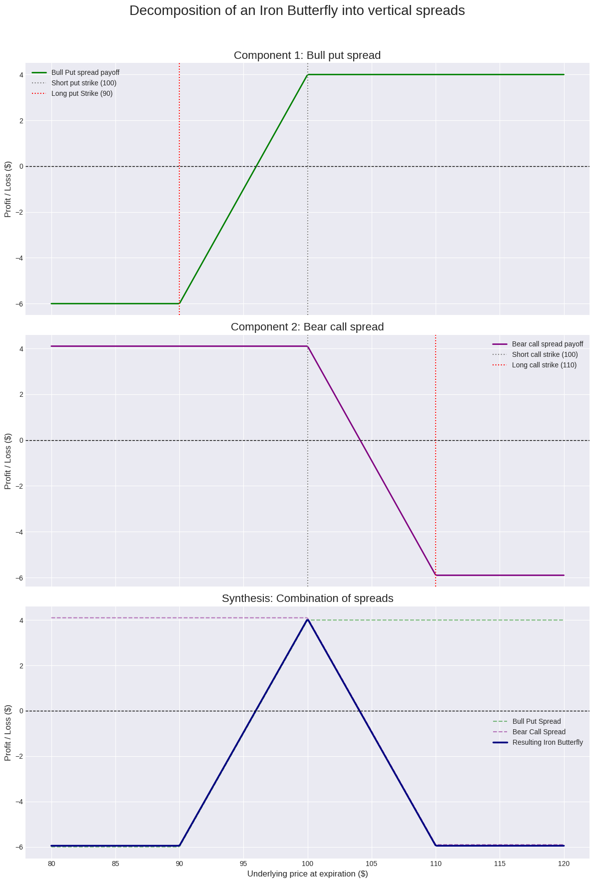
Before we model the dynamics of the Iron Butterfly, we must first understand its static anatomy. The strategy is a composite structure. It is synthetically equivalent to the combination of two distinct vertical credit spreads: a Bear Call Spread and a Bull Put Spread. Understanding these "atomic" components provides a more granular view of the risk being assumed.

A vertical spread involves the simultaneous purchase and sale of two options of the same type (calls or puts) and same expiration, but with different strike prices.

1. The bear call spread:

   A bear call spread is a credit spread constructed by selling a call option and buying another call option with a higher strike price. It represents a bearish to neutral bet. The trader profits if the underlying stays below the short call strike, collecting the net premium. The long call serves to cap the maximum loss if the price rallies significantly.

   \(\begin{aligned} \textbf{Construction:}\quad &\text{Sell }C\bigl(K_{\mathrm{short}}\bigr)\;+\;\text{Buy }C\bigl(K_{\mathrm{long}}\bigr), \quad K_{\mathrm{long}}>K_{\mathrm{short}},\\[6pt] \textbf{Net premium received:}\quad &P \;=\; C\bigl(K_{\mathrm{short}}\bigr)\;-\;C\bigl(K_{\mathrm{long}}\bigr),\\[6pt] \textbf{Max profit:}\quad &\Pi_{\max} \;=\; P,\quad\text{realized if }S_{T}\le K_{\mathrm{short}},\\[6pt] \textbf{Max loss:}\quad &\Pi_{\min} \;=\;\bigl(K_{\mathrm{long}}-K_{\mathrm{short}}\bigr)\;-\;P, \quad\text{realized if }S_{T}\ge K_{\mathrm{long}}. \end{aligned}\)

2. The bull put spread:

   A bull put spread is a credit spread constructed by selling a put option and buying another put option with a lower strike price. It represents a bullish to neutral bet. The trader profits if the underlying stays above the short put strike. The long put caps the maximum loss if the price falls sharply.

   \(\begin{aligned} \textbf{Construction:}\quad &\text{Sell }P\bigl(K_{\mathrm{short}}\bigr)\;+\;\text{Buy }P\bigl(K_{\mathrm{long}}\bigr), \quad K_{\mathrm{long}}<K_{\mathrm{short}},\\[6pt] \textbf{Net premium received:}\quad &P_{\mathrm{net}} \;=\; P\bigl(K_{\mathrm{short}}\bigr)\;-\;P\bigl(K_{\mathrm{long}}\bigr),\\[6pt] \textbf{Max profit:}\quad &\Pi_{\max} \;=\; P_{\mathrm{net}}, \quad\text{realized if }S_{T}\ge K_{\mathrm{short}},\\[6pt] \textbf{Max loss:}\quad &\Pi_{\min} \;=\;\bigl(K_{\mathrm{short}}-K_{\mathrm{long}}\bigr)\;-\;P_{\mathrm{net}}, \quad\text{realized if }S_{T}\le K_{\mathrm{long}}. \end{aligned}\)

3. Synthesis of the iron butterfly:

   The Iron Butterfly emerges from the simultaneous sale of an at-the-money (or near-the-money) bear call spread and bull put spread, where the short strikes are the same.

   \(\begin{aligned} \text{Iron Butterfly} &= \bigl(\text{Sell }C(K_{S}) \;+\; \text{Buy }C(K_{LC})\bigr) + \bigl(\text{Sell }P(K_{S}) \;+\; \text{Buy }P(K_{LP})\bigr)\\ &= \text{Bear Call Spread} \;+\; \text{Bull Put Spread} \end{aligned}\)

   This decomposition reveals that the total risk of the Iron Butterfly is the sum of the risks of its constituent spreads. The negative delta from the Bear Call Spread initially offsets the positive delta from the Bull Put Spread, creating a delta-neutral position. The negative gamma from both short options combines to create the deep gamma trough at the center of the butterfly.

   Let's visualize this decomposition.

   

Pillar 1 - Stochastic underlier dynamics

The first step is to acknowledge that the underlying asset does not follow a simple path. The Black-Scholes-Merton model's assumption of a log-normal distribution for asset prices is a useful starting point, but it fails to capture two critical empirical facts:

1. Volatility clustering (the tendency for high-volatility periods and low-volatility periods to group together).

2. Price jumps.

To build a more realistic model, we combine two ideas:

1. The Heston model for stochastic volatility.

2. The Merton model for jump-diffusion.

The Heston-Jump model describes the evolution of the asset price (S_t​) and its variance (ν_t​) with the following system of stochastic differential equations:

\(\begin{align*} dS_t &= \mu\,S_t\,dt + \sqrt{v_t}\,S_t\,dW^1_t,\\ dv_t &= \kappa\bigl(\theta - v_t\bigr)\,dt + \sigma\,\sqrt{v_t}\,dW^2_t. \end{align*}\)

Here:

• μ is the risk-free rate.

• ν_t​​ is the instantaneous variance.

• κ is the rate of mean reversion of the variance.

• θ is the long-term mean of the variance.

• σ is the volatility of the variance (the vol of vol).

• dW_t¹ and dW_t​²​ are Wiener processes with correlation ρ, i.e., E[dW_t¹ ​dW_t​²​]=ρdt. The correlation ρ is crucial for capturing the leverage effect (typically ρ<0).

The Merton jump-diffusion model adds discontinuous jumps to the asset price path:

\(\frac{dS_t}{S_t} = (\mu - \lambda k)\,dt + \sigma\,dW_t + dJ_t.\)

where J_t​ is a compound Poisson process, λ is the average number of jumps per year, and k is the average jump size.

Combining these gives us a Heston-Jump model. Pricing options under such a model is non-trivial as there is no simple closed-form solution like Black-Scholes. Instead, we turn to Fourier transform methods. The price of a European call option can be calculated by integrating the characteristic function of the log-asset price. The Fang-Oosterlee COS method provides a highly efficient and accurate way to do this by using a Fourier-cosine series expansion of the probability density function.

Let's implement the characteristic function for the Heston-Jump model. This function is essential for pricing via the COS method.

import numpy as np
from scipy.stats import norm

# --- Heston-Jump Model Characteristic Function ---
# This function is the mathematical core for pricing options under a sophisticated model
# that accounts for both stochastic volatility (Heston) and price jumps (Merton).
def heston_jump_char_func(u, T, r, v0, theta, kappa, sigma, rho, muJ, sigmaJ, lambda_jump):
    """
    Calculates the characteristic function for the Heston-Jump model.
    
    Args:
        u (complex): The argument of the characteristic function.
        T (float): Time to maturity.
        r (float): Risk-free rate.
        v0 (float): Initial variance.
        theta (float): Long-term variance.
        kappa (float): Mean-reversion speed of variance.
        sigma (float): Volatility of variance ('vol of vol').
        rho (float): Correlation between asset price and variance.
        muJ (float): Mean of the log jump size.
        sigmaJ (float): Standard deviation of the log jump size.
        lambda_jump (float): Intensity of the Poisson jump process.
        
    Returns:
        complex: The value of the characteristic function.
    """
    i = 1j
    
    # Heston part
    d = np.sqrt((kappa - i * rho * sigma * u)**2 + (sigma**2) * (u**2 + i * u))
    g = (kappa - i * rho * sigma * u - d) / (kappa - i * rho * sigma * u + d)
    
    C = (kappa * theta) / (sigma**2) * ((kappa - i * rho * sigma * u - d) * T - 2 * np.log((1 - g * np.exp(-d * T)) / (1 - g)))
    D = ((kappa - i * rho * sigma * u - d) / (sigma**2)) * ((1 - np.exp(-d * T)) / (1 - g * np.exp(-d * T)))
    
    phi_heston = np.exp(C + D * v0)
    
    # Jump part (Merton)
    # The jump compensator ensures the process is a martingale under the risk-neutral measure
    compensator = lambda_jump * (np.exp(muJ + 0.5 * sigmaJ**2) - 1)
    phi_jump = np.exp(T * lambda_jump * (np.exp(i * u * muJ - 0.5 * u**2 * sigmaJ**2) - 1))
    
    # Combined characteristic function
    phi = phi_heston * phi_jump
    
    # Final term with interest rate and drift adjustment
    return np.exp(i * u * (r - compensator) * T) * phi

def generate_paths():
    T = 1.0  # 1 year
    N_STEPS = 252
    N_PATHS = 1
    dt = T / N_STEPS
    S0 = 100
    r = 0.02

    # GBM parameters
    sigma_gbm = 0.20
    
    # Heston-Jump parameters
    v0 = 0.04  # Initial variance (20% vol)
    theta = 0.04 # Long-term variance
    kappa = 2.0  # Mean-reversion speed
    sigma_v = 0.3 # Vol of vol
    rho = -0.7 # Correlation
    
    # Jump parameters
    lambda_j = 0.5 # 0.5 jumps per year on average
    mu_j = -0.1 # Average jump size (log)
    sigma_j = 0.15 # Jump size volatility

    # Generate paths
    gbm_path = np.zeros(N_STEPS + 1)
    hj_path = np.zeros(N_STEPS + 1)
    gbm_path[0] = S0
    hj_path[0] = S0
    v_t = v0

    for t in range(1, N_STEPS + 1):
        # Standard Wiener processes
        Z1 = norm.rvs()
        Z2 = norm.rvs()
        W1 = np.sqrt(dt) * Z1
        W2 = np.sqrt(dt) * (rho * Z1 + np.sqrt(1 - rho**2) * Z2)
        
        # GBM Path
        gbm_path[t] = gbm_path[t-1] * np.exp((r - 0.5 * sigma_gbm**2) * dt + sigma_gbm * W1)
        
        # Heston-Jump Path
        # Euler discretization for variance (with full truncation to ensure positivity)
        v_t = v_t + kappa * (theta - v_t) * dt + sigma_v * np.sqrt(max(v_t, 0)) * W2
        v_t = max(v_t, 0)
        
        # Jump component
        poisson_draw = np.random.poisson(lambda_j * dt)
        jump = 0
        if poisson_draw > 0:
            jump = np.random.normal(mu_j, sigma_j) * poisson_draw
            
        hj_path[t] = hj_path[t-1] * np.exp((r - 0.5 * v_t) * dt + np.sqrt(v_t) * W1 + jump)

    return gbm_path, hj_path

gbm, hj = generate_paths()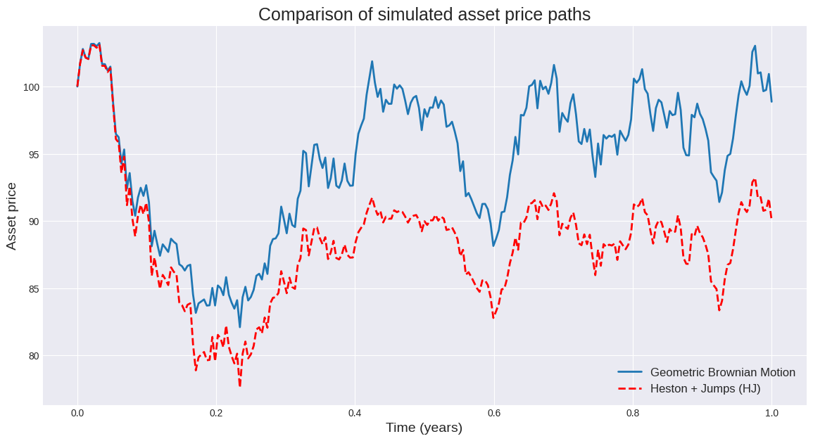

The plot clearly illustrates the inadequacy of the simple GBM model. The Heston-Jump path exhibits periods of changing volatility and, most importantly, a significant discontinuous jump. An Iron Butterfly strategy priced and risked on the smooth GBM path would be completely unprepared for the reality of the HJ path. Adopting a more sophisticated underlying model is the non-negotiable first pillar of a robust system.

Pillar 2: Volatility surface parameterisation

The characteristic function from Pillar 1 allows us to price an option for a single maturity and strike, given a set of model parameters. The real world, however, presents us with a whole surface of option prices across all available strikes and expiries. The implied volatility (IV) extracted from these prices is not flat; it forms a "smile" or "skew." Our model must be able to replicate this surface consistently. This process is called calibration.

A naive approach of calibrating the Heston-Jump model to every single option would be computationally infeasible for real-time trading. Instead, we use a parametric model for the volatility surface itself. One of the industry standards is the Stochastic Volatility Inspired (SVI) model, proposed by Gatheral in 2004. The SVI formula parameterizes the total implied variance w=σ²_BS​T as a function of log-moneyness k=log(K/F), where K is the strike and F is the forward price.

The raw SVI formula for a single slice of the volatility smile is:

\(w(k) = a + b\left\{ \rho\,(k - m) \;+\; \sqrt{(k - m)^2 + \sigma^2} \right\}.\)

The parameters {a,b,ρ,m,σ} control the level (a), the slope (ρ), the curvature (b), the at-the-money position (m), and the rounding of the vertex (σ) of the smile.

A key requirement for any volatility model is that it must not allow for static arbitrage. Specifically, the price of a butterfly spread (C(K−ΔK)−2C(K)+C(K+ΔK)) must be non-negative. This translates into a condition on the second derivative of the call price with respect to the strike, which in turn imposes constraints on the SVI parameters. Gatheral and Jacquier showed the necessary and sufficient no-butterfly-arbitrage conditions for SVI.

To handle jumps, the SVI model can be extended to SVI-J, which embeds a jump intensity term λ_J​. The calibration process then involves finding the set of SVI-J parameters that minimizes the squared error between the model's implied volatilities and the market's implied volatilities, typically weighted by the options' vega.

This is a non-linear optimization problem, perfectly suited for JIT compilation frameworks like Google's JAX. It allows us to write the objective function in pure Python and then automatically compute its gradient.

import jax
import jax.numpy as jnp
from jax import jit, grad

# --- SVI-J volatility smile calibration ---
# This demonstrates how to calibrate an SVI model to market data.
# SVI is a powerful way to parameterize the vol smile, and JAX makes the
# optimization process incredibly efficient.

@jit
def svi_raw(k, params):
    """SVI raw variance formula."""
    a, b, rho, m, sigma = params
    return a + b * (rho * (k - m) + jnp.sqrt((k - m)**2 + sigma**2))

# Let's assume we have some market data (log-moneyness and implied vols)
# In a real scenario, this would come from a live data feed.
market_log_moneyness = jnp.array([-0.2, -0.1, 0.0, 0.1, 0.2])
market_implied_vols = jnp.array([0.25, 0.22, 0.20, 0.21, 0.24])
T = 1.0 # 1 year maturity
market_total_variance = market_implied_vols**2 * T

def loss_function(params):
    """
    Calculates the sum of squared errors between the SVI model
    and market variances. This is the function we want to minimize.
    """
    model_total_variance = svi_raw(market_log_moneyness, params)
    return jnp.sum((model_total_variance - market_total_variance)**2)

# Use JAX to get the gradient of the loss function
grad_loss = jit(grad(loss_function))

# --- Simple Gradient Descent optimization ---
# Initial guess for parameters [a, b, rho, m, sigma]
# A good initial guess is crucial for convergence.
initial_params = jnp.array([0.04, 0.1, -0.5, 0.0, 0.1]) 
learning_rate = 0.01
n_iterations = 2000

params = initial_params
for i in range(n_iterations):
    gradients = grad_loss(params)
    params -= learning_rate * gradients
    # In a real implementation, we would add constraints to ensure
    # the parameters are valid (e.g., b >= 0, |rho| < 1).

print("Calibrated SVI parameters:", params)

fine_log_moneyness = jnp.linspace(-0.3, 0.3, 100)
calibrated_variance = svi_raw(fine_log_moneyness, params)
calibrated_vols = jnp.sqrt(calibrated_variance / T)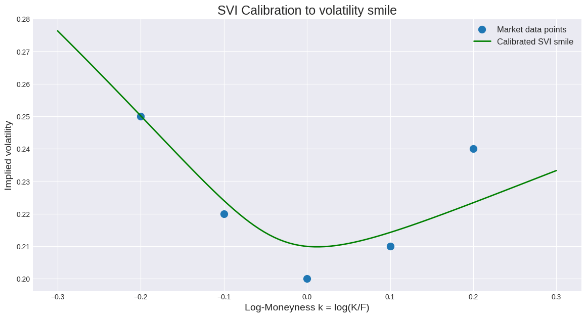

A common misconception is that one can simply linearly interpolate implied volatilities between strikes. This is demonstrably false and dangerous. Linear interpolation of IV does not guarantee the absence of arbitrage. It is possible to construct butterfly spreads using linearly interpolated values that have a negative cost but a non-negative payoff, a free lunch. The SVI parameterization, when correctly constrained, explicitly enforces the necessary convexity (no-butterfly-arbitrage) to ensure a consistent and arbitrage-free representation of the volatility surface. This is not an academic point; it is a prerequisite for any serious options modeling.

Pillar 3: Payoff geometry and dynamic greek trajectories

With a calibrated model, we can now analyze the risk of our Iron Butterfly. As you already know from the previous article the Greeks are the partial derivatives of the option price with respect to various parameters. Don’t forget to check it in more detail here:

[WITH CODE] Options: Iron Condor

For a this strategy, they are the key to understanding its dynamic behavior.

\(\begin{aligned} \Delta &= \frac{\partial V}{\partial S}: \text{Sensitivity to a change in the underlying price. }\\ \Gamma &= \frac{\partial^2 V}{\partial S^2}: \text{Sensitivity of Delta to a change in the underlying price.}\\ \nu &= \frac{\partial V}{\partial \sigma}: \text{Sensitivity to a change in implied volatility.}\\ \Theta &= \frac{\partial V}{\partial t}: \text{Sensitivity to the passage of time.} \end{aligned}\)

From here we derive:

1. An Iron Butterfly is initiated delta-neutral.

2. The Iron Butterfly is short Gamma, which is the source of its risk.

3. The Iron Butterfly is short Vega.

4. The Iron Butterfly is long Theta, which is its primary source of profit.

The Greeks are not static. Their evolution is governed by a set of partial differential equations. For example, the change in Delta over time is not zero, even if the price doesn't move:

\(\frac{d\Delta}{dt} = \frac{\partial \Delta}{\partial t} + \frac{\partial \Delta}{\partial S}\,\frac{dS}{dt} + \frac{\partial \Delta}{\partial \sigma}\,\frac{d\sigma}{dt}.\)

This expands to include higher-order Greeks:

\(\frac{d\Delta}{dt} \approx \Theta_{\Delta}\,dt +\Gamma\,dS +\mathrm{Vanna}\,\cdot d\sigma.\)

where Vanna (∂Δ​/∂σ) measures the change in delta for a change in volatility. This shows that your delta hedge is not stable. It changes with time, price moves, and volatility changes. A robust algorithm must continuously monitor and manage these dynamic trajectories.

Let's visualize this payoff and its key Greeks.

import numpy as np
from scipy.stats import norm

# --- Black-Scholes Pricer and Greeks ---
# For illustration, we'll use Black-Scholes, but in a real system,
# the pricer from Pillar 1 would be used.
def black_scholes_greeks(S, K, T, r, sigma, option_type='call'):
    d1 = (np.log(S / K) + (r + 0.5 * sigma**2) * T) / (sigma * np.sqrt(T))
    d2 = d1 - sigma * np.sqrt(T)
    
    if option_type == 'call':
        price = S * norm.cdf(d1) - K * np.exp(-r * T) * norm.cdf(d2)
        delta = norm.cdf(d1)
    else: # put
        price = K * np.exp(-r * T) * norm.cdf(-d2) - S * norm.cdf(-d1)
        delta = norm.cdf(d1) - 1
        
    gamma = norm.pdf(d1) / (S * sigma * np.sqrt(T))
    theta = -(S * norm.pdf(d1) * sigma) / (2 * np.sqrt(T)) - r * K * np.exp(-r * T) * norm.cdf(d2) if option_type == 'call' else \
            -(S * norm.pdf(d1) * sigma) / (2 * np.sqrt(T)) + r * K * np.exp(-r * T) * norm.cdf(-d2)
            
    return price, delta, gamma, theta

def iron_butterfly_profile(S_range, K_short, K_long_put, K_long_call, T, r, sigma):
    # Short ATM Straddle + Long OTM Strangle
    # Short Call at K_short, Short Put at K_short
    # Long Put at K_long_put, Long Call at K_long_call
    
    # Prices
    p_short_call, d_sc, g_sc, t_sc = black_scholes_greeks(S_range, K_short, T, r, sigma, 'call')
    p_short_put,  d_sp, g_sp, t_sp = black_scholes_greeks(S_range, K_short, T, r, sigma, 'put')
    p_long_put,   d_lp, g_lp, t_lp = black_scholes_greeks(S_range, K_long_put, T, r, sigma, 'put')
    p_long_call,  d_lc, g_lc, t_lc = black_scholes_greeks(S_range, K_long_call, T, r, sigma, 'call')
    
    # Total P&L, Delta, Gamma, Theta
    pnl = -p_short_call - p_short_put + p_long_put + p_long_call
    delta = -d_sc - d_sp + d_lp + d_lc
    gamma = -g_sc - g_sp + g_lp + g_lc
    theta = -t_sc - t_sp + t_lp + t_lc
    
    return pnl, delta, gamma, theta

# --- Parameters ---
S0 = 100
K_short = 100
wing_width = 10
K_long_put = K_short - wing_width
K_long_call = K_short + wing_width
T = 30/365 # 30 days to expiration
r = 0.02
sigma = 0.20

S_range = np.linspace(S0 - wing_width*2, S0 + wing_width*2, 200)

# Calculate profiles
pnl_initial, delta, gamma, theta = iron_butterfly_profile(S_range, K_short, K_long_put, K_long_call, T, r, sigma)
pnl_expiration = np.minimum(np.maximum(S_range - K_long_put, 0), wing_width) - np.minimum(np.maximum(S_range - K_short, 0), wing_width)
pnl_expiration = (pnl_expiration - np.mean(pnl_expiration)) # Simplified payoff shape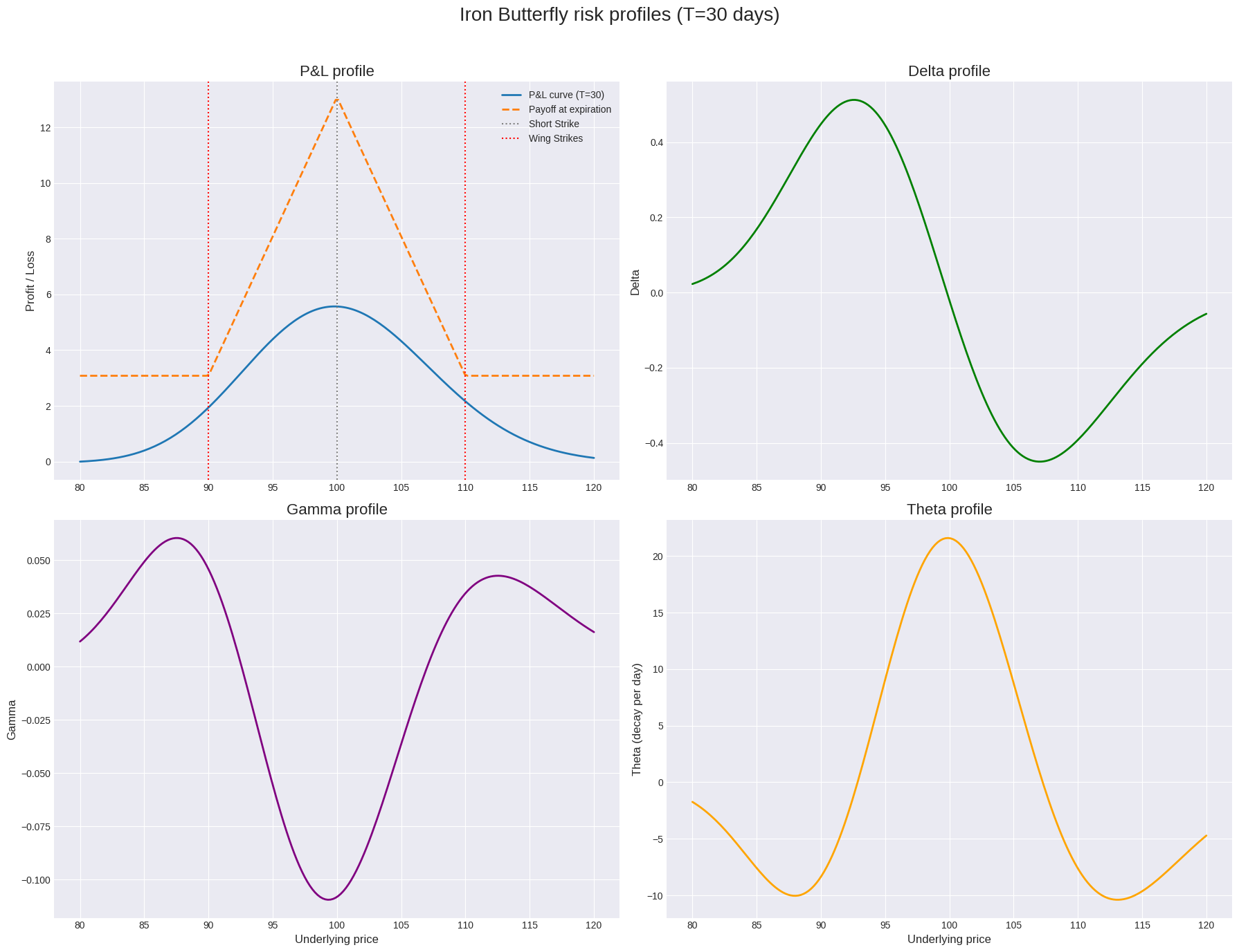

The plots reveal the classic risk structure. The PnL curve shows the tent shape. The Gamma plot shows a deep negative trough centered at the short strike, meaning we lose money at an accelerating rate as the price moves away from the center. The Theta plot is the mirror image, showing that our maximum time decay profit occurs when the underlying is stable.

A critical misconception is to focus solely on the Gamma value at the current price. The real danger is the integrated effect of Gamma over a large price move. The Gamma risk is quadratic inside the wings but becomes linear outside them. Hedging based only on the local Gamma at the ATM strike dramatically underestimates the risk of a large, gapping move that jumps into the wings. This is because the Delta of the position changes almost linearly with price once the underlying is outside the short strikes, leading to a slope-dominated blow-up risk. A sophisticated algorithm must manage its risk based on the entire Gamma profile, not just a single point estimate.

Pillar 4: Execution micro-structure heuristics

Having a perfect model of the market is useless if you cannot transact in it efficiently. The field of optimal execution deals with the problem of how to place large orders with minimal cost. The classic institutional model in this space is from Almgren and Chriss but feel free to choose an approach that adjusts better to your Butterfly’s set up.

They model the cost of trading as a combination of two factors:

1. Permanent market impact (your trading permanently shifts the equilibrium price).

2. Temporary market impact (your trading creates a temporary price pressure that dissipates after you stop trading).

The goal is to liquidate a portfolio of X shares over a time horizon T by choosing a trading trajectory v(t)=dx/dt​ that minimizes the expected cost, while also penalizing the variance (risk) of that cost. This leads to a calculus of variations problem, the solution of which is an exponential curve. The optimal strategy is to trade faster at the beginning and slow down as you approach the deadline.

The temporary impact cost for a trade of size q_i​ at time i can be modeled as

\(\eta(q_i) \;=\; \epsilon\,\operatorname{sgn}(q_i)\;+\;\gamma\,q_i.\)

where ϵ is a fixed cost and γ is the linear impact coefficient. The Almgren-Chriss model provides a framework for solving the trade-off between the risk of holding the position longer (price may move against you) and the cost of executing too quickly (high market impact).

Let's simulate an optimal execution trajectory using the Almgren-Chriss framework. We need to solve a differential equation that describes the optimal trading rate.

from scipy.integrate import odeint

# --- Almgren-Chriss Optimal Execution ---
# This code solves for the optimal liquidation path to minimize a combination
# of execution costs and volatility risk.

def almgren_chriss_ode(y, t, k, eta):
    """The ODE system for the Almgren-Chriss model."""
    # y[0] is h(t), y[1] is h'(t)
    return [y[1], k**2 * y[0]]

# Parameters
T = 1.0  # Liquidation horizon (e.g., 1 day)
X = 10000  # Total shares to liquidate
sigma = 0.3  # Volatility
eta = 2.5e-7 # Temporary market impact parameter
gamma = 2.5e-7 # Permanent market impact parameter
lambd = 1e-6 # Risk aversion parameter

# Derived parameters for the ODE
k = np.sqrt(lambd * sigma**2 / eta)

# Solve the ODE
t_space = np.linspace(0, T, 50)
# The solution to the ODE is of the form A*cosh(kt) + B*sinh(kt)
# We solve for h(T)=0 and h'(T)=0 to find the trading trajectory v(t)
# The analytical solution for the trading rate v(t) is:
v_t = (2 * k * X * np.exp(k * (T - t_space))) / (np.exp(2 * k * T) - 1) * np.cosh(k * (T - t_space))
# A simpler form is often used:
v_t_simple = (X * k * np.cosh(k * (T - t_space))) / np.sinh(k * T)


# Calculate the inventory remaining
x_t = np.zeros_like(t_space)
x_t[0] = X
for i in range(1, len(t_space)):
    x_t[i] = x_t[i-1] - v_t_simple[i-1] * (t_space[i] - t_space[i-1])
x_t[-1] = 0 # Ensure it ends at zero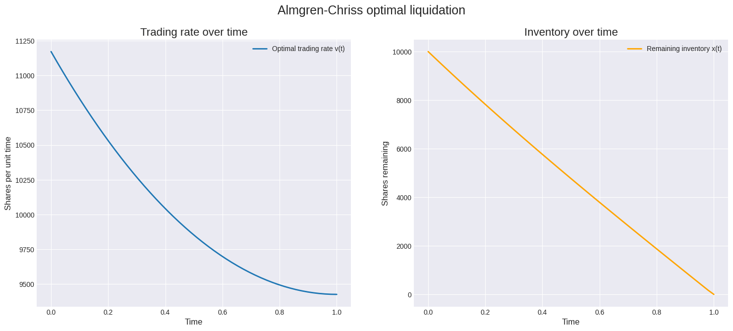

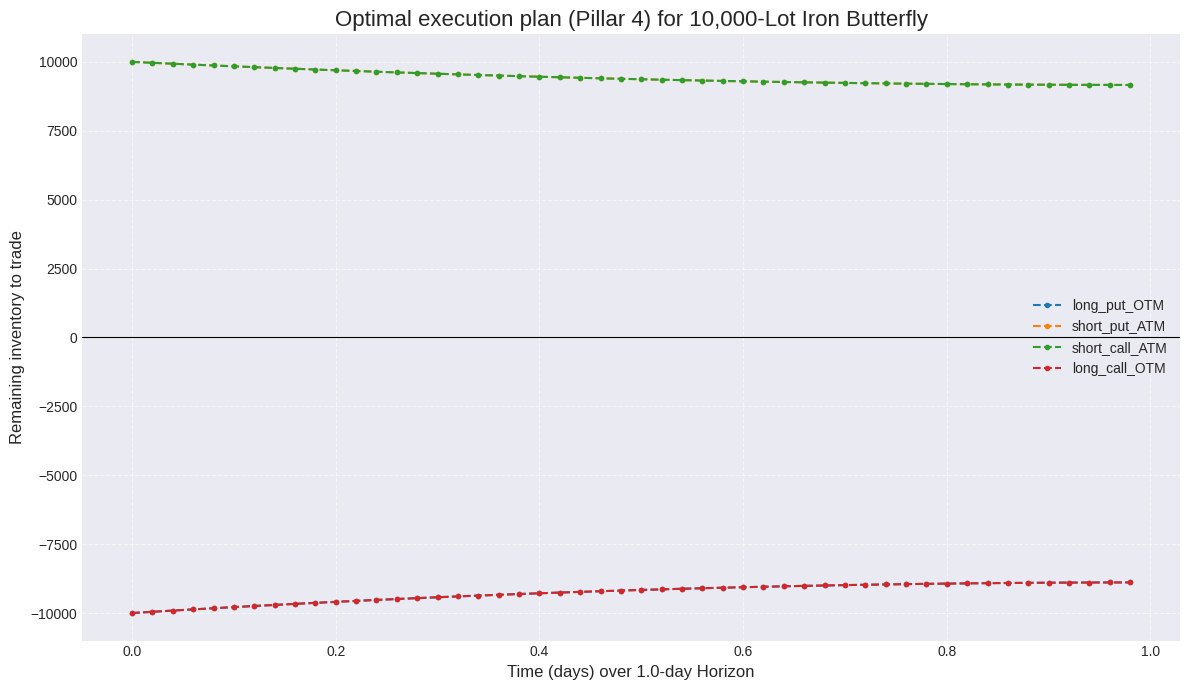
The plots show the characteristic shape of the optimal strategy. The trading rate is highest at the beginning and decays exponentially, while the inventory depletes along a corresponding curve. For an Iron Butterfly, this logic applies to all four legs simultaneously, and also to the continuous delta-hedging that must occur throughout the life of the trade.

The common industry benchmarks of TWAP (Time-Weighted Average Price) and VWAP (Volume-Weighted Average Price) are fundamentally naive. They are passive, deterministic strategies that completely ignore market conditions, risk, and information leakage. Believing that a TWAP execution is "neutral" is an illusion; it is simply a bet that the price will follow a straight line, an assumption that is rarely true. True neutrality comes from an optimal, risk-aware execution strategy.

Pipeline automatization

The script you have in the appendix functions as a complete, automated pipeline that models the workflow of the strategy, from initial analysis to final execution planning. The process begins by defining all the necessary parameters for a potential Iron Butterfly trade:

1. This initial setup is immediately fed into an analytical engine, which represents the first major phase of the pipeline. Using the Black-Scholes model, this engine calculates the trade's fundamental financial profile—its maximum potential profit, maximum loss, and the resulting risk-to-reward ratio. Crucially, this analysis isn't just for human review; it's for an automated decision engine.

2. The script checks the calculated metrics against a predefined set of rules, such as a minimum acceptable risk-to-reward ratio. If the trade fails to meet these criteria, the pipeline automatically halts, deeming the trade not worth pursuing. If it's approved, the system performs a deeper dive, generating a detailed table of the position's risk characteristics (its Greeks) across a range of prices and simulating a calibration of the volatility surface.

Once a trade has been analyzed and approved, the pipeline seamlessly transitions to the execution planning phase. This step addresses the practical challenge of how to actually place the four separate orders in the market with minimal cost.

The final output of the pipeline is a comprehensive report that includes all the data from the analysis and decision steps.

Pretty nifty, huh!? All right, team—stellar effort today! The Iron Butterfly might look like a tighter, “precision” version of the Condor, but don’t be fooled into thinking it’s a walk in the park. That slim profit zone between your short strikes demands razor-sharp analytics: options Greeks, probability distributions, dynamic hedging, and code that can react to every tick. In an algorithmic framework, you’re building models that estimate tail-risk, calibrate implied vols, backtest entry/exit rules, and even automate adjustments on the fly.

So remember: there’s no magic “set-and-sleep” switch here. Every Iron Butterfly you place is backed by calculus, statistics, and lines of code. Now it’s time to power down and recharge those neurons—tomorrow, we return with fresh charts, fresh curiosity, and that ever-hungry quant mindset. Keep probing, keep coding, keep the quant flame burning! Stay quanty! 🖥️

---

👍🏻 If you liked the article and are interested in this topic, feel free to join our discussion group!

---

PS: What brances of statistics would you like to see in the Quant Lectures section?

Appendix

The full script

from __future__ import annotations

import math
from dataclasses import dataclass, field
from typing import Callable, Dict, Tuple

import numpy as np
import pandas as pd
from scipy.stats import norm
import matplotlib.pyplot as plt

# ==============================================================================
# SECTION 1: DATACLASSES & UTILITIES
# ==============================================================================
@dataclass
class TradeParams:
    """All parameters defining the iron butterfly trade and models."""
    qty: int
    spot: float
    r: float
    # Strikes
    K_low: float
    K_mid: float
    K_high: float
    # Time
    T_trade: float  # Time to expiration for options (Pillar 3)
    T_exec: float   # Time horizon for execution (Pillar 4)
    N_exec: int     # Number of execution steps
    # Market Impact (Pillar 4)
    eta: float
    gamma: float
    # Volatility (used across pillars)
    vol_atm: float   # ATM Volatility for body
    vol_wing: float  # OTM Volatility for wings (smile effect)

@dataclass
class AnalysisReport:
    """Holds all results from the analysis phase."""
    is_approved: bool
    reason: str
    net_credit: float = 0.0
    max_profit: float = 0.0
    max_loss: float = 0.0
    risk_reward_ratio: float = 0.0
    breakevens: Tuple[float, float] = (0, 0)
    greek_profile: pd.DataFrame = field(default_factory=pd.DataFrame)
    svi_params: Tuple = ()


# ==============================================================================
# SECTION 2: CORE PILLAR IMPLEMENTATIONS
# ==============================================================================

# ---------------------------------------------------------------------------
# Pillar 4 –– Almgren–Chriss primitives
# ---------------------------------------------------------------------------
@dataclass
class ACParams:
    sigma: float; eta: float; gamma: float; T: float; N: int; X: float

class AlmgrenChrissSolver:
    def __init__(self, params: ACParams, risk_aversion: float):
        self.p = params
        self.lambda_ = float(risk_aversion)

    def get_schedule(self) -> pd.DataFrame:
        p, dt, k = self.p, self.p.T / self.p.N, math.sqrt(self.lambda_ * self.p.sigma**2 / self.p.eta)
        x = np.linspace(p.X, 0, p.N + 1) if math.isclose(k, 0) else \
            p.X * np.cosh(k * (p.T - np.arange(p.N + 1) * dt)) / np.cosh(k * p.T)
        v = -np.diff(x) / dt
        return pd.DataFrame({"t": np.linspace(0, p.T, p.N, endpoint=False), "inventory": x[:-1], "trade_rate": v})

# ---------------------------------------------------------------------------
# Pillar 2 –– Raw-SVI slice calibrator
# ---------------------------------------------------------------------------
def svi_raw(k: np.ndarray, params: Tuple) -> np.ndarray:
    a, b, rho, m, sig = params
    return a + b * (rho * (k - m) + np.sqrt((k - m)**2 + sig**2))

def calibrate_svi(k: np.ndarray, total_var: np.ndarray) -> Tuple:
    params = np.array([0.04, 0.1, -0.4, 0.0, 0.1], dtype=float)
    for _ in range(2000):
        w = svi_raw(k, params)
        res, (_, b, rho, m, sig) = 2 * (w - total_var), params
        st = np.sqrt((k - m)**2 + sig**2)
        grads = [np.sum(res), np.sum(res * (rho * (k - m) + st)), np.sum(res * b * (k - m)),
                 np.sum(res * b * (-rho - (k - m) / st)), np.sum(res * b * (sig / st))]
        params -= 0.01 * np.array(grads) / len(k)
    return tuple(params)

# ---------------------------------------------------------------------------
# Pillar 3 –– Greek engine (using Black-Scholes as the pricer)
# ---------------------------------------------------------------------------
def _bs_pricer(S: float | np.ndarray, K: float, T: float, r: float, sigma: float, kind: str) -> Dict:
    S_arr, d1 = np.asarray(S, dtype=float), (np.log(S / K) + (r + 0.5 * sigma**2) * T) / (sigma * np.sqrt(T))
    d2 = d1 - sigma * np.sqrt(T)
    if kind == "call":
        price, delta = S_arr * norm.cdf(d1) - K * np.exp(-r * T) * norm.cdf(d2), norm.cdf(d1)
        theta = -(S_arr * norm.pdf(d1) * sigma) / (2 * np.sqrt(T)) - r * K * np.exp(-r * T) * norm.cdf(d2)
    else:
        price, delta = K * np.exp(-r * T) * norm.cdf(-d2) - S_arr * norm.cdf(-d1), norm.cdf(d1) - 1
        theta = -(S_arr * norm.pdf(d1) * sigma) / (2 * np.sqrt(T)) + r * K * np.exp(-r * T) * norm.cdf(-d2)
    gamma = norm.pdf(d1) / (S_arr * sigma * np.sqrt(T))
    return {"price": price, "delta": delta, "gamma": gamma, "theta": theta}

class IronButterflyGreeks:
    def __init__(self, p: TradeParams, pricer: Callable = _bs_pricer):
        self.p, self._pricer = p, pricer

    def get_profile(self, S_range: np.ndarray) -> pd.DataFrame:
        p = self.p
        g = lambda K, kind: self._pricer(S_range, K, p.T_trade, p.r, p.vol_atm, kind)
        short_put, short_call = g(p.K_mid, 'put'), g(p.K_mid, 'call')
        long_put, long_call = g(p.K_low, 'put'), g(p.K_high, 'call')
        
        delta = long_put['delta'] - short_put['delta'] - short_call['delta'] + long_call['delta']
        gamma = long_put['gamma'] - short_put['gamma'] - short_call['gamma'] + long_call['gamma']
        theta = long_put['theta'] - short_put['theta'] - short_call['theta'] + long_call['theta']
        
        return pd.DataFrame({'S': S_range, 'delta': delta, 'gamma': gamma, 'theta': theta})


# ==============================================================================
# SECTION 3: AUTOMATED PIPELINE ORCHESTRATION
# ==============================================================================

def run_analysis_and_decision(p: TradeParams, decision_config: Dict) -> AnalysisReport:
    """Runs Pillars 1, 2, 3 and the decision engine."""
    # --- Pillar 3: P&L Analysis ---
    pricer_args = {"S": p.spot, "T": p.T_trade, "r": p.r, "sigma": p.vol_atm}
    price = lambda K, kind: _bs_pricer(K=K, kind=kind, **pricer_args)['price']
    
    net_credit = price(p.K_mid, 'put') + price(p.K_mid, 'call') - price(p.K_low, 'put') - price(p.K_high, 'call')
    
    if net_credit <= 0:
        return AnalysisReport(is_approved=False, reason="Trade results in a net debit.")

    max_profit = net_credit * p.qty
    max_loss = (p.K_mid - p.K_low - net_credit) * p.qty
    risk_reward = max_profit / max_loss if max_loss > 0 else float('inf')
    breakevens = (p.K_mid - net_credit, p.K_mid + net_credit)

    # --- Decision Engine ---
    if risk_reward < decision_config["min_risk_reward_ratio"]:
        reason = f"Risk/Reward {risk_reward:.2f} is below threshold {decision_config['min_risk_reward_ratio']:.2f}"
        return AnalysisReport(is_approved=False, reason=reason)
    
    # --- Pillar 3: Generate full Greek Profile (if approved) ---
    S_range = np.linspace(p.K_low * 0.95, p.K_high * 1.05, 51)
    greek_engine = IronButterflyGreeks(p)
    greek_profile = greek_engine.get_profile(S_range)
    
    # --- Pillar 2: Calibrate Volatility Surface (demonstration) ---
    k = np.linspace(-0.2, 0.2, 11)
    market_iv = p.vol_atm * (1 + 0.5 * k**2 - 0.3 * k) # Mock smile
    market_total_var = market_iv**2 * p.T_trade
    svi_params = calibrate_svi(k, market_total_var)

    return AnalysisReport(
        is_approved=True, reason="Trade approved by all criteria.",
        net_credit=net_credit, max_profit=max_profit, max_loss=max_loss,
        risk_reward_ratio=risk_reward, breakevens=breakevens,
        greek_profile=greek_profile, svi_params=svi_params
    )

def run_execution(p: TradeParams, risk_aversion: float) -> Dict[str, pd.DataFrame]:
    """Runs Pillar 4 to generate execution schedules."""
    legs = {
        "long_put_OTM":   {'X': -p.qty, "sigma": p.vol_wing},
        "short_put_ATM":  {'X': p.qty,  "sigma": p.vol_atm},
        "short_call_ATM": {'X': p.qty,  "sigma": p.vol_atm},
        "long_call_OTM":  {'X': -p.qty, "sigma": p.vol_wing},
    }
    schedules = {}
    for name, overrides in legs.items():
        ac_p = ACParams(eta=p.eta, gamma=p.gamma, T=p.T_exec, N=p.N_exec, **overrides)
        schedules[name] = AlmgrenChrissSolver(ac_p, risk_aversion).get_schedule()
    return schedules

def run_automated_pipeline():
    """Main function to run the full analysis-to-execution pipeline."""
    # 1. DEFINE TRADE & PIPELINE PARAMETERS
    print("[STEP 1/4] Defining trade & pipeline parameters")
    params = TradeParams(
        qty=10_000, 
        spot=100.0, 
        r=0.05,
        K_low=90.0, 
        K_mid=100.0, 
        K_high=110.0,
        T_trade=30/365, 
        T_exec=1.0, N_exec=50,
        eta=5e-7, 
        gamma=2e-7,
        vol_atm=0.30, 
        vol_wing=0.35,
    )
    decision_config = {"min_risk_reward_ratio": 0.15}
    risk_aversion = 1e-6
    print("Parameters defined successfully.\n")

    # 2. RUN ANALYSIS & DECISION ENGINE (PILLARS 2 & 3)
    print("[STEP 2/4] Running analysis & decision engine")
    report = run_analysis_and_decision(params, decision_config)
    
    if not report.is_approved:
        print(f"EXECUTION HALTED. Reason: {report.reason}")
        return

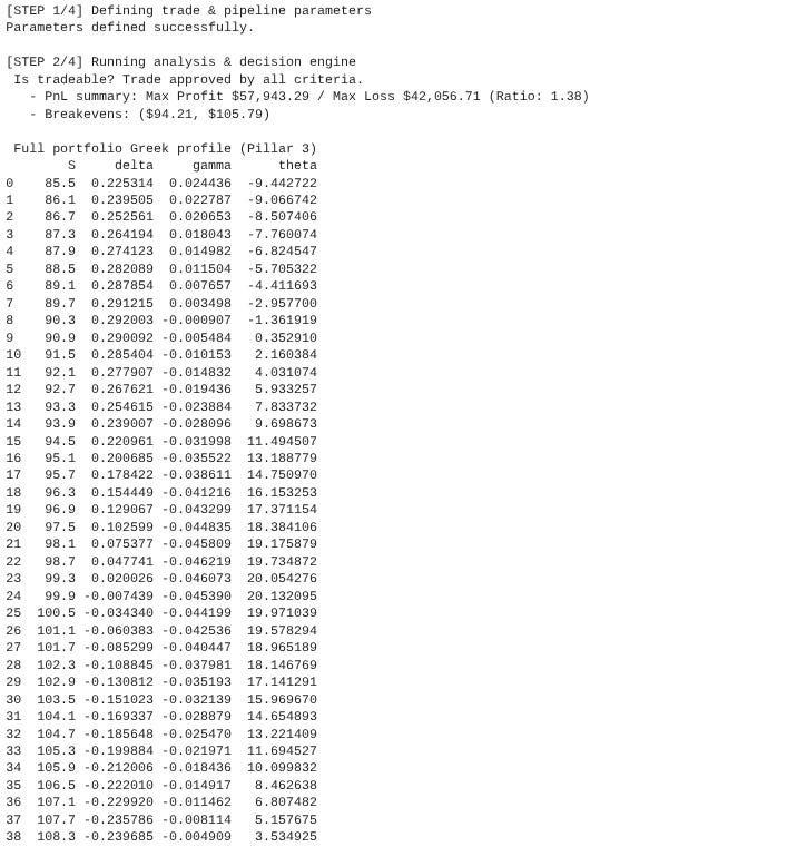
    print(f" Is tradeable? {report.reason}")
    print(f"   - PnL summary: Max Profit ${report.max_profit:,.2f} / Max Loss ${report.max_loss:,.2f} (Ratio: {report.risk_reward_ratio:.2f})")
    print(f"   - Breakevens: (${report.breakevens[0]:.2f}, ${report.breakevens[1]:.2f})")
    
    print("\n Full portfolio Greek profile (Pillar 3)")
    print(report.greek_profile.to_string())

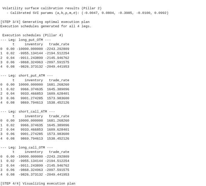
    print("\n\n Volatility surface calibration results (Pillar 2)")
    print(f"   - Calibrated SVI params (a,b,ρ,m,σ): ({', '.join(f'{x:.4f}' for x in report.svi_params)})\n")

    # 3. GENERATE EXECUTION PLAN (PILLAR 4)
    print("[STEP 3/4] Generating optimal execution plan")
    schedules = run_execution(params, risk_aversion)
    print("Execution schedules generated for all 4 legs.")

    print("\n Execution schedules (Pillar 4)")
    for name, schedule in schedules.items():
        print(f"--- Leg: {name} ---")
        print(schedule.head())
        print()
        
    # 4. VISUALIZE EXECUTION PLAN
    print("[STEP 4/4] Visualizing execution plan")
    fig, ax = plt.subplots(figsize=(12, 7))
    for name, schedule in schedules.items():
        ax.plot(schedule['t'], schedule['inventory'], marker='.', linestyle='--', label=name)
    ax.set_title(f"Optimal execution plan (Pillar 4) for {params.qty:,}-Lot Iron Butterfly", fontsize=16)
    ax.set_xlabel(f"Time (days) over {params.T_exec}-day Horizon", fontsize=12)
    ax.set_ylabel("Remaining inventory to trade", fontsize=12)
    ax.grid(True, linestyle='--', alpha=0.6)
    ax.legend()
    ax.axhline(0, color='black', linewidth=0.8)
    fig.tight_layout()
    plt.show()

# Run the entire pipeline
if __name__ == "__main__":
    run_automated_pipeline()