
Trading the Breaking

Trading the Breaking

Research

[WITH CODE] Infra: Free data from Tradingview

Download all the data from TradingView’s servers for $0.

May 25, 2026
∙ Paid

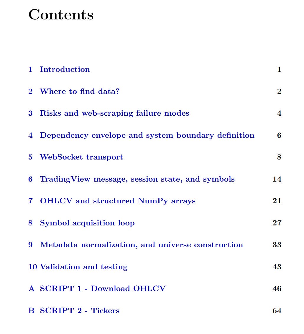
Table of contents:

  1. Introduction.

  2. Where to find data?

  3. Risks and web-scraping failure modes.

  4. Dependency envelope and system boundary definition.

  5. WebSocket transport.

  6. TradingView message, session state, and symbols.

  7. OHLCV and structured NumPy arrays.

  8. Symbol acquisition loop.

  9. Metadata normalization, and universe construction.


Audio Note: Before we begin, remember that if you’re accessing this article through the Substack app, you can listen to it instead of reading it.

Before you begin, remember that you have an index with the newsletter content organized by clicking on the image below.


Introduction

Algorithmic trading begins with a data question before it becomes a model question. Every signal, backtest, risk estimate, execution assumption, and portfolio rule depends on the historical record that feeds the system. A strategy is a function of its data. When the data source changes, the object under study changes with it.

Independent researchers face this problem under capital constraints. Market data subscriptions, platform limits, and research time compete for the same budget. Everybody knows how hard is to find a profitable strategy so traders may need data before premium infrastructure becomes affordable. However, the researcher needs enough historical evidence to test an idea before expanding spending.

Free data has value. It gives the researcher access, speed, breadth, and experimentation capacity. Its risk profile comes from the conditions attached to that access. Endpoint changes, rate limits, missing fields, symbol inconsistencies, session conventions, adjustment modes, and partial responses can enter the research process as hidden assumptions.

The practical answer is to stop treating acquisition as a casual download. This builds a small research stack around that idea. One part retrieves OHLCV bars from TradingView. The other builds the symbol universe that feeds those requests. The code stays close to the source, so the researcher can see how raw access becomes a structured object for testing.

From there, the workflow becomes research-ready. The researcher can trace the source path, preserve the request logic, validate the output, and understand which data conventions shape the sample before the first model decision occurs.

Where to find data?

The first question in algorithmic trading concerns data origin. The question comes before model choice. A trading strategy is a function over a historical record. When that record contain unstable fields, adjustment errors, or hidden provider changes, the strategy test becomes unstable.

Independent traders enter the problem from a cash constraint. They seek cheap data because the platform account, broker margin, hosting, and research time consume capital. Paying hundreds per month for a data subscription before a strategy proves itself creates an uncomfortable sequence. The market still imposes the same standard. A weak data feed can make a bad strategy look acceptable, make a decent strategy look broken, and hide a good idea under avoidable noise. Free data can be true. The core difficulty is that free data comes with weak evidence about error conditions.

Premium data reduces many operational risks and keeps responsibility on the researcher. A paid feed may provide service-level agreements, corporate-action files, delisting history, explicit licensing, historical corrections, and support channels. Those advantages have economic value because they reduce unknowns. The premium label still has to match the strategy. A daily equity strategy needs corporate-action logic. A futures strategy needs roll methodology. A foreign-exchange strategy needs session boundaries. An intraday strategy needs timezone, holiday, daylight-saving, and microstructure details. A paid vendor can deliver observations that are correct in format and wrong in use.

The trader needs research data before institutional data becomes affordable. The correct response is to treat free data as a constrained research source with documented guarantees and documented gaps. The trader gets data from an available source, then records what that source can guarantee and what it leaves uncertain.

Algorithmic trading contains many arguments about alpha built on casual data pipelines. Alpha is a small signal estimated inside a noisy environment. A two-basis-point edge can vanish through timestamp leakage, holiday mismatch, stale universe selection, or a split adjustment imported after the backtest export. The data layer defines the sample and which trades could have existed. When the sample is wrong, the alpha estimate describes a different object.

Risks and web-scraping failure modes

The uncomfortable truth is that a data pipeline is one of the sources of model risk. In algorithmic trading, the market data loader is part of the strategy, even when it looks like infrastructure. A bad entry signal is easy to blame. A silent data defect is harder.

Free data carries a different risk profile. The visible risks are rate limits, endpoint changes, missing values, duplicated bars, inconsistent symbol formats, unavailable historical depth, and provider-side throttling. Indeed, a free source can return adjusted close with raw open, split-adjusted prices with incomplete dividend treatment, or bars whose volume semantics differ across markets. It can omit delisted names, creating a survivorship-biased universe that looks stronger than the universe available at the time. It can make calendars look aligned because the stored sample contains successful requests and much more.

Let’s look at some of these risks in more detail:

  1. The first limitation is protocol fragility. The script handles the WebSocket layer: socket creation, TLS wrapping, HTTP upgrade, WebSocket masking, ping/pong responses, frame parsing, TradingView packet packing, and ~m~<length>~m~<payload> message extraction. This is technically strong because it avoids third-party dependencies, but it also means the script depends on message conventions that may change without warning.

    A premium data vendor normally gives an official API contract: documented fields, deprecation policy, status pages, versioned endpoints, and support. A scraped or reverse-engineered feed gives none of that. If TradingView changes a header requirement, modifies the session protocol, renames a method, changes the packet envelope, throttles unauthenticated requests, or alters how heartbeats behave, the script may stop working.

  2. The second limitation is rate limits, throttling and sampling bias. The ticker scanner already includes a pause argument between paginated requests. That is a design decision that reduces aggressive request behavior and lowers the probability of rate-limit problems. In fact, it can create sampling bias.

  3. The final limitation is the most important, web-scraped or unofficially acquired data is usually not execution-grade by default. Execution-grade data needs stronger guarantees: timestamp precision, exchange-specific calendars, correction handling, corporate-action methodology, symbol mapping, delisting coverage, latency expectations, outage reporting, and licensing clarity. The current scripts are useful for acquisition and research, but they do not yet implement a full institutional data stack.

Dependency envelope and system boundary definition

In a research stack, every dependency is implicit. A wrapper library may save time, but it can also hide protocol assumptions, retry behavior, schema changes, rate-limit responses, and timestamp conversions. In this case, we chose a narrow dependency envelope so the researcher can see what happens between the socket and the structured array.

The purpose of a minimal acquisition layer is to reduce the number of unknown transformations between the remote data source. In market data, unknown transformations are expensive:

  • Did the wrapper adjust for splits?

  • Did it include dividends?

  • Did it localize timestamps?

  • Did it align sessions?

  • Did it forward-fill missing volume?

  • Did it retry after a failed request and mix partial data into a final table?

The less visible the path, the more forensic work is required when a strategy behaves too well.

The header of the OHLCV script names the supported output. A dictionary mapping TradingView symbols such as NASDAQ:AAPL or TVC:VIX to structured NumPy arrays with datetime, open, high, low, close, and volume fields. That output is the first useful data model in the project. This makes the next stage of research straightforward because every downstream function can rely on named fields and stable numeric dtypes.

# SCRIPT 1 - OHLCV
TV_HOST = "data.tradingview.com"
TV_PATH = "/socket.io/websocket"
TV_ORIGIN = "https://www.tradingview.com"

Portability across vendors should be built at the interface, not faked inside the source adapter. This script is a source adapter. It should speak TradingView’s language and then emit a local object with a stable schema. The right boundary is therefore a small function that returns arrays in a controlled dtype. A separate layer can later convert those arrays into pandas, Polars, Arrow, Parquet, a feature store, or a database. Mixing the vendor protocol and the research table abstraction too early would make the system harder to test.

When a library wrapper fails, you often see only the wrapper exception. Here, the possible failures are closer to the actual layers—DNS or socket creation, TLS wrapping, WebSocket upgrade, frame serialization or a TradingView message. That is more work, but it gives a better map where debugging becomes easier.

The second script uses the same philosophy but applies it to ticker extraction. It imports json, time, urllib.request, and urllib.error. The scanner client therefore depends on the standard library rather than requests. The script wants to POST JSON to a known scanner endpoint, receive JSON back, and build dictionaries. Nothing about that requires a large HTTP stack. If later the user needs sessions, proxies, rotating headers, backoff middleware, caching, or async dispatch, those can be added.

# SCRIPT 2 - Tickers
import json
import time
import urllib.request
import urllib.error

TV_SCANNER_BASE_URL = "https://scanner.tradingview.com"

The data script starts when the universe is defined.

WebSocket transport

The WebSocket portion is the most technically interesting part of the OHLCV script. It opens a TCP connection, wraps it with TLS, creates a Sec-WebSocket-Key, writes the HTTP upgrade request, reads the upgrade response, and checks for the 101 status. Many researchers never see this layer because websocket-client or a vendor SDK does it for them. Here it is visible, and that visibility is useful because the data feed is a stream with a handshake, framing rules, liveness behavior, and failure states.

The function _ws_connect is the gatekeeper. If it fails, there is no chart session, no symbol resolution, and no bars. In production, this function is part of the availability budget. If a research script runs once per day, failure is annoying. If a scanner-plus-fetcher runs across thousands of symbols, even a small connection failure probability becomes a measurable drag on data completeness. A proper acquisition engine would count connection attempts, upgrade failures, elapsed time, remote closes, and timeout frequency. The current function raises clear errors, which is a good starting point.

def _ws_connect(timeout: int = 20):
    raw_sock = socket.create_connection((TV_HOST, 443), timeout=timeout)
    ctx = ssl.create_default_context()
    sock = ctx.wrap_socket(raw_sock, server_hostname=TV_HOST)

    key = base64.b64encode(os.urandom(16)).decode()
    request = (
        f"GET {TV_PATH} HTTP/1.1\r\n"
        f"Host: {TV_HOST}\r\n"
        "Upgrade: websocket\r\n"
        "Connection: Upgrade\r\n"
        f"Sec-WebSocket-Key: {key}\r\n"
        "Sec-WebSocket-Version: 13\r\n"
        f"Origin: {TV_ORIGIN}\r\n"
        "User-Agent: Mozilla/5.0\r\n"
        "\r\n"
    )
    sock.sendall(request.encode())

That makes the TradingView dependency obvious and exposes the browser-like headers. If TradingView changes accepted headers, this is where the break will happen.

The next important design point is frame masking. WebSocket clients must mask frames sent to the server. The _ws_send_text function constructs the frame header, chooses the correct payload-length encoding, generates a random four-byte mask, applies it byte by byte, and sends the final frame. This is the kind of code that looks low-level for a research workflow, but it is exactly the level at which many unofficial data clients break when protocol assumptions drift.

This implementation is compact and correct for basic text frames. It implements the WebSocket behavior needed for this research task. For a batch OHLCV downloader, that boundary is appropriate. The researcher understands that the code targets the data-download workflow rather than the full surface area of a general-purpose WebSocket library, including fragmentation, compression extensions, advanced close-code handling, and reconnect state.

def _ws_send_text(sock, text: str):
    payload = text.encode("utf-8")
    length = len(payload)

    header = bytearray()
    header.append(0x81)  # FIN + text frame

    if length <= 125:
        header.append(0x80 | length)
    elif length < 65536:
        header.append(0x80 | 126)
        header += struct.pack(">H", length)
    else:
        header.append(0x80 | 127)
        header += struct.pack(">Q", length)

    mask = os.urandom(4)
    masked_payload = bytes(payload[i] ^ mask[i % 4] for i in range(length))
    sock.sendall(header + mask + masked_payload)

The mask is required for client-to-server frames. If this function is wrong, the failure can look like a remote-side refusal even though the symbol, interval, and TradingView method are all valid.

The receive side is equally important. The function _ws_recv_text reads two bytes, extracts the opcode, checks the payload length, optionally unmasks the payload, handles close frames, responds to pings with pongs, ignores pongs, and returns text frames.

The script’s ping-pong handling is a strength because many quick data clients ignore it. In a cross-sectional downloader, slow symbols, large n_bars values, and network jitter make liveness important. The code treats the stream as a conversation rather than a one-way file download.

def _ws_recv_text(sock) -> str:
    while True:
        b1, b2 = _recv_exact(sock, 2)
        opcode = b1 & 0x0F
        masked = b2 & 0x80
        length = b2 & 0x7F

        if length == 126:
            length = struct.unpack(">H", _recv_exact(sock, 2))[0]
        elif length == 127:
            length = struct.unpack(">Q", _recv_exact(sock, 8))[0]

        mask = _recv_exact(sock, 4) if masked else None
        payload = _recv_exact(sock, length) if length else b""

        if opcode == 0x8:
            raise ConnectionError("TradingView closed the WebSocket.")
        if opcode == 0x9:
            _ws_send_pong(sock, payload)
            continue
        if opcode == 0x1:
            return payload.decode("utf-8", errors="ignore")

It suppresses control-frame noise and returns only text payloads to the TradingView parser. This separation keeps the higher-level OHLCV function focused on messages such as timescale update and series completed.

The current script raises or prints errors in sensible places, but a production research engine should turn those errors into events. A CSV or JSON log with symbol, interval, n_bars, error class, elapsed seconds, attempt number, and returned bar count would make data acquisition auditable.

TradingView message, session state, and symbols

Once the WebSocket is alive, the helper _tv_pack wraps a JSON payload inside the TradingView envelope format (a marker, the payload length, another marker, and the JSON body). The length prefix is key because TradingView can send multiple logical messages inside a single WebSocket text frame, and the client needs a deterministic way to separate them.

The _extract_tv_packets function is therefore a core parser. It scans the accumulated buffer for the envelope marker, reads the declared payload length, waits if the current buffer is incomplete, and returns complete packets with a residual buffer. This is the kind of logic that prevents subtle parse corruption. If the client assumes one socket frame equals one TradingView message, it will work until it does not. When it fails, the error will look random. A truncated JSON object, a missing series update, or a swallowed heartbeat. The script avoids that by treating the TradingView envelope as the true unit of protocol state.

def _tv_pack(method: str, params: list) -> str:
    payload = json.dumps({"m": method, "p": params}, separators=(",", ":"))
    return f"~m~{len(payload)}~m~{payload}"


def _extract_tv_packets(buffer: str):
    packets = []
    pos = 0
    while True:
        start = buffer.find("~m~", pos)
        if start == -1:
            return packets, ""
        len_start = start + 3
        len_end = buffer.find("~m~", len_start)
        if len_end == -1:
            return packets, buffer[start:]
        length_str = buffer[len_start:len_end]
        if not length_str.isdigit():
            pos = len_end + 3
            continue
        payload_len = int(length_str)
        payload_start = len_end + 3
        payload_end = payload_start + payload_len
        if len(buffer) < payload_end:
            return packets, buffer[start:]
        packets.append(buffer[payload_start:payload_end])
        pos = payload_end

The session layer begins with _random_session, which generates identifiers such as cs_xxxxxxxxxxxx. This is more than a convenience. TradingView chart sessions multiplex state. The downloader creates a chart session, resolves a symbol within that session, and creates a series attached to that symbol. The random suffix makes a session identifier collision unlikely, but the key point is conceptual. The requested bars are a stateful resource. The client builds a stateful context and then asks the server to stream a series update.

The main get_tradingview_ohlcv function sends messages in a sequence that makes sense, like set_auth_token, chart_create_session, resolve_symbol, create_series.

_tv_send(sock, "set_auth_token", ["unauthorized_user_token"])
_tv_send(sock, "chart_create_session", [chart_session, ""])

resolved_symbol = _symbol_payload(
    symbol=symbol,
    session=session,
    adjustment=adjustment,
)

_tv_send(sock, "resolve_symbol", [chart_session, "symbol_1", resolved_symbol])
_tv_send(sock, "create_series", [
    chart_session,
    series_id,
    series_id,
    "symbol_1",
    interval,
    int(n_bars),
])

The complete request goes beyond a ticker string. It includes a session mode, an adjustment mode, an interval, and a bar count. In our research, those fields define the dataset and belong with the downloaded array.

The symbol payload function deserves special attention because it exposes two parameters that directly affect conclusions—session and adjustment. Session defines whether the data uses regular or extended trading hours. Adjustment defines whether prices are adjusted for splits, dividends, or left raw. These choices are research-defining inputs. A moving-average strategy, volatility estimate, overnight return study, breakout rule, or volume filter can change materially depending on regular-session versus extended-session bars and split-adjusted versus raw prices.

The script defaults to regular session and splits adjustment. That is a defensible default for many equity research tasks because it avoids some discontinuities caused by stock splits while keeping pre-market and after-hours activity separate from regular bars. The convention still needs to be documented. When a strategy shows edge, the first reviewer should ask “edge under which session and adjustment convention?” A reproducible backtest records that answer clearly.

def _symbol_payload(symbol: str, session: str = "regular", adjustment: str = "splits") -> str:
    payload = {
        "symbol": symbol,
        "adjustment": adjustment,
        "session": session,
    }
    return "=" + json.dumps(payload, separators=(",", ":"))

Adjustment mode defines the price process being modeled. Let Ct​ be the close at time t. A split-adjusted close Ctadj​ is a different stochastic process from a raw close Ctraw​. A return model usually requires continuity through corporate actions, so it often uses adjusted data. An execution simulator uses raw tradable prices and handles corporate actions. The script can request different adjustment modes, so the research layer records the adjustment convention as metadata attached to each array.

\(r_t = \log\left(\frac{C_t}{C_{t-1}}\right), \qquad C_t \in \left\{ C_t^{\mathrm{raw}},\, C_t^{\mathrm{split\text{-}adj}},\, C_t^{\mathrm{dividend\text{-}adj}} \right\}\)

The equation is simple, but it is enough to invalidate a backtest when ignored. A split in raw data creates a large negative return that does not represent an economic loss. A split-adjusted series removes that discontinuity for return research. Dividend adjustment introduces another explicit convention. The script’s flexibility is valuable because it supports these different conventions, and the metadata makes that flexibility reproducible. A useful extension returns both the structured array and a small metadata object containing source, symbol, interval, n_bars, session, adjustment, request_time_utc, and downloader_version.

Send me a copy

OHLCV and structured NumPy arrays

The parser _parse_timescale_update turns TradingView's timescale_update payload into a list of numeric tuples. The function expects bars with a vector v containing timestamp, open, high, low, close, and possibly volume. It skips bars with fewer than five values and sets volume to np.nan if volume is absent. This is one of the best practical decisions in the script. Missing volume remains missing rather than being converted to zero. Zero volume is a statement, missing volume is uncertainty. Preserving that distinction avoids a common retail-data mistake.

A zero-volume bar can mean no volume, depending on the instrument and venue. A missing volume field means the source did not provide the value in that message. Those are different observations. In algorithmic trading, volume feeds liquidity filters, execution-cost models, volatility scaling, breakout confirmation, and regime classification. Treating missing volume as zero can falsely classify a liquid symbol as untradable or distort turnover constraints. Using np.nan preserves the distinction and forces downstream code to decide how to handle the missing value.

def _parse_timescale_update(msg: dict, series_id: str):
    try:
        payload = msg["p"][1]
        series = payload.get(series_id, {})
        bars = series.get("s", [])
    except Exception:
        return []

    out = []
    for bar in bars:
        values = bar.get("v", [])
        if len(values) < 5:
            continue

        timestamp = float(values[0])
        open_ = float(values[1])
        high = float(values[2])
        low = float(values[3])
        close = float(values[4])
        if len(values) >= 6 and values[5] is not None:
            volume = float(values[5])
        else:
            volume = np.nan

The next function, _bars_to_array, defines the local schema. It creates a structured NumPy dtype with datetime64 seconds and float64 fields for open, high, low, close, and volume. The timestamp conversion uses integer seconds and casts to datetime64[s]. This is compact and efficient. It also avoids the overhead of a DataFrame at the source boundary.

A structured array is serializable, typed, compact, and easy to validate. DataFrames are excellent for research manipulation, but they can hide dtype drift. A structured array forces this schema. In a larger system, one could convert to a DataFrame after validation.

dtype = [
    ("datetime", "datetime64[s]"),
    ("open", "f8"),
    ("high", "f8"),
    ("low", "f8"),
    ("close", "f8"),
    ("volume", "f8"),
]

arr = np.zeros(len(bars), dtype=dtype)
arr["datetime"] = timestamps.astype("datetime64[s]")
arr["open"] = [b[1] for b in bars]
arr["high"] = [b[2] for b in bars]
arr["low"] = [b[3] for b in bars]
arr["close"] = [b[4] for b in bars]
arr["volume"] = [b[5] for b in bars]

The minimum validation layer around this array should enforce OHLC inequalities. For each bar, low should not exceed open, high, or close. High should not be below open, low, or close. Prices should be finite and positive for standard equities, indices, and spot FX rates. Timestamps should increase after sorting, unless the source returns reverse chronological data and the script normalizes it. The current code does not perform these checks, but it is okay for the moment.

\(\mathrm{low}_t \le \min(\mathrm{open}_t, \mathrm{close}_t) \le \max(\mathrm{open}_t, \mathrm{close}_t) \le \mathrm{high}_t \)

A violated OHLC bar can break volatility estimates, range features, candlestick rules, stop-loss simulations, and intrabar execution assumptions. One corrupted high can create a false breakout. One negative close can explode logarithmic returns. One non-monotonic timestamp can produce lookahead when arrays are joined across assets. The array function should remain simple, but the caller should immediately pass the output through a validator.

The validation snippet looks like this:

This post is for paid subscribers

Already a paid subscriber? Sign in
© 2026 Quant Beckman · Publisher Privacy ∙ Publisher Terms
Substack · Privacy ∙ Terms ∙ Collection notice
Start your SubstackGet the app
Substack is the home for great culture