


Table of contents:
Introduction.
The role of ETL in the design of trading systems.
ETL failure modes and risks.
Technical preliminaries.
Designing an ETL.
Layers, contracts and canonical schema.
ETL vs ELT for trading.
What breaks ETL in trading systems.
Before you begin, remember that you have an index with the newsletter content organized by clicking on “Read the newsletter index” in this image.

Introduction
We enter the part of the quant stack that drives everything: data. We treat data as the machinery that tells a trading system what the market is—minute by minute, venue by venue, revision by revision.
This new serie introduces a sequence of articles on infrastructure—ETLs, scraping, APIs—written from the quant-dev perspective: trading systems need repeatable market states. Research needs to recreate yesterday. Live trading needs to ingest today. Both need to refer to the same definitions.
A familiar pattern shows up in almost every desk, prop shop, or solo setup. Data starts as a handful of scripts, then grows into a maze of just this once fixes: a quick endpoint here, a patched column there, a notebook cell that becomes a dependency because it worked during a good backtest. The system still runs. Results still appear. But the pipeline becomes a moving object—shifting definitions, shifting assumptions, shifting outputs—until the only thing that remains stable is confusion.
That is why ETL deserves a dedicated article. The reason? A pipeline accumulates decisions: what gets stored, what gets normalized, what gets ignored, what gets re-requested, what gets overwritten, what gets trusted… Those decisions compound, and at some point they dominate the behavior of the entire stack. The strategy stops being the bottleneck. The data becomes the bottleneck.
")
Scraping and APIs deserve equal attention because they are how most modern trading pipelines actually exist in the wild. They impose constraints, quirks, and failure patterns: response truncation, pagination inconsistencies, silent field changes, intermittent outages, caching surprises, and vendor helpfulness.
The goal across this series is to make data infrastructure feel less like maintenance and more like a controlled instrument. A good pipeline behaves like a well-specified system: deterministic when it should be deterministic, conservative when it must be conservative, and transparent when something deviates.
Check this paper to know more about ETLs:
So the promise of this article is concrete. By the end, it becomes natural to answer questions that otherwise stay vague: Where did this feature come from? Which definition did it use? When did it change? Can the dataset be recreated byte-for-byte? What happens when the vendor revises history? How does the system fail when the feed degrades? Those are operational questions, but they decide whether research can be trusted and whether live behavior can be diagnosed.
The role of ETL in the design of trading systems
Three components are typically treated as core in any trading system: strategy logic, execution, and risk. The ETL process—Extract, Transform, Load—is often categorized as a secondary support function. However, this categorization understates the structural role ETL plays in defining the parameters of the trading environment. It is the ETL process that establishes timestamp semantics and interval conventions, just as it defines the mechanics of volume aggregation across venues, determines the handling of missing prints or stale quotes, and establishes the boundaries of the trading day, including the definition of market close during partial sessions or under vendor-specific conventions.
A weak data pipeline permits a model to stay numerically consistent even when it lacks economic coherence. This failure manifests as an epistemic mismatch. The model trains on information unavailable at the time of execution or on data representations that drift between the training environment and the live feed. Backtests appear profitable but lack causal validity. Live trading degradation follows as a predictable consequence of this architecture.

Scale makes ETL automation a key pillar. But it is a challenge that requires automating the whole process. That means, new failures. From a quant dev perspective, this presents a tension between three competing criteria: velocity, correctness, and observability. Velocity is necessary because research iteration and feature publication are time-sensitive. Correctness is critical because a single semantic mismatch can introduce systematic lookahead bias without any explicit error in the code. Observability is essential because, without reproducibility and data lineage, it is impossible to distinguish between a failure of strategy logic and a failure of data construction. Once models are trained on warehouse-ready features, the ETL pipeline becomes an implicit component of the model itself.

ETL failure modes and risks
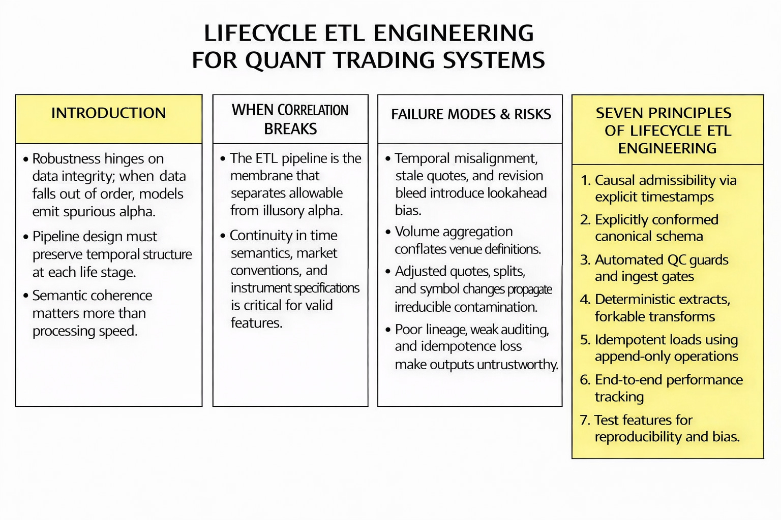
ETL failure modes exist across domains, but in trading they are amplified because signals are marginal and backtests are sensitive to subtle causal violations. It is useful to name the principal failure modes, as a map from data defects to PnL leakage.
Temporal integrity risk is the most frequent source of silent contamination. Timezone normalization errors—exchange time, broker server time, and UTC being conflated—create misalignment that can masquerade as alpha. Bar timestamp conventions are often ambiguous: some providers label bars by start time, others by end time, and others by a vendor-defined label that is neither. DST discontinuities can duplicate or remove hourly timestamps. APIs frequently return date fields with implicit timezones. Resampling without explicit session calendars can manufacture bars during market closures. None of these defects need an explicit future reference to introduce lookahead, misalignment is sufficient.
Market microstructure risk emerges when sampling and aggregation rules are treated as interchangeable. For example, volume is venue-specific; cross-venue volume is not additive unless definitions match. VWAP computed from incomplete trade prints is not VWAP. OHLC bars from heterogeneous vendors can be numerically similar while being non-equivalent, which means return distributions can look stable while microstructure features drift. Mixing bid/ask and last-trade series destroys interpretability of returns, spread-sensitive features, and execution assumptions. Even quote filtering—removing stale quotes or enforcing spread constraints—changes the effective sampling distribution and can alter feature–target dependence.
Firm actions and instrument definition risk is where many useless backtests are born. Splits, dividends, symbol changes, roll schedules for futures, and specification changes in tick size or lot size all require explicit treatment. A toxic pattern is using adjusted close alongside raw open/high/low, which creates a synthetic object with inconsistent scale.
Data leakage risk is the highest-impact failure mode because it converts structural error into apparent predictive power. Vendor revisions—late prints, corrected OHLC—can enter historical features without an as-of policy. Using the close price for signals intended to be decided at open changes the filtration. Filling missing values using future data is leakage by construction. End-of-day fundamentals used for intraday signals without controlling for publication time inject future information. Even innocuous preprocessing, such as z-scoring using full-sample statistics, can leak information when deployed online.
Heterogeneity risk is both schema and semantics. NaN encodings differ across sources (null, zero, empty string). Identical field names can have different meaning, as when volume is shares, contracts, or notional. Data types differ and can change silently (float versus decimal, integer timestamps versus ISO strings). Precision and rounding differences can alter microstructure-sensitive computations and create spurious stability.
Operational risk appears when automation is treated as job finished equals success. Cron jobs can succeed while returning partial data. API rate limits can truncate responses. Network errors can create gaps, retries can create duplicates. Incremental loads can fail to be idempotent. Failures often cluster on holidays, early closes, vendor maintenance windows, and schedule drift that causes overlapping extraction windows.
Heavy transformations performed repeatedly inside modelling loops change the feasible hypothesis class. Recomputing features that should be materialized wastes iteration budget and induces inconsistent definitions when code evolves. Unbounded joins across large fact tables can make the research loop unstable under scaling.
Technical preliminaries
Trading doesn’t tolerate imprecise definitions because PnL is sensitive to small causal misalignments. Let Pt denote a price process under an explicit convention (bid, ask, mid, last). Let Vt denote an associated volume process with explicit units (shares, contracts, notional). Let It denote the sigma-algebra of information available up to time t. A trading signal St must be It-measurable.
An ETL pipeline can be modeled as a composition of maps,
where ε extracts from raw sources into an event stream, T transforms into conformed representations, and L loads into storage layers (OLTP and DW).
Online transaction processing (OLTP) is a type of database system used in transaction-oriented applications, such as many operational systems. Online refers to the fact that such systems are expected to respond to user requests and process them in real-time (process transactions). The term is contrasted with online analytical processing (OLAP) which instead focuses on data analysis (for example planning and management systems).
Data warehouse (DW), is a system used for reporting and data analysis and is a core component of goberning. Data warehouses are central repositories of data integrated from disparate sources.
The critical property is causal admissibility. For any feature Ft used at decision time t, Ft must be measurable with respect to It. ETL violates this property through mechanisms that look operationally reasonable: aggregations that use end-of-window values while decisions occur at window start; imputation via centered filters; backfills that overwrite previously published features without version control; and “helpful” resampling rules that use future ticks to fill an OHLC bar.
This is why causal admissibility must be enforced by automated tests. If the system can’t prove the property, the property doesn’t hold operationally.
To remove ambiguity, define three timelines. Observation time t(e) (event-time) is when the market produced the observable. Processing time t(p) is when the system ingested it. Decision time t(d) is when the strategy commits to an action.
A bar at index k has an interval [tk,start , tk,end). If a strategy acts at bar open, then tk(d) . Features must not depend on events with t(e)≥tk,start.
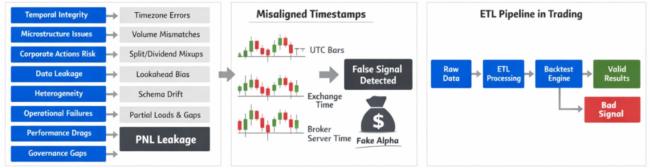
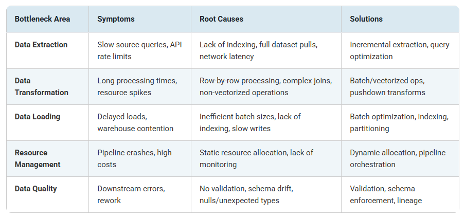
Before diving into more complex staff, understanding where ETL pipelines typically struggle helps prioritize improvement efforts. Here’s a breakdown of common bottleneck areas:
Designing an ETL
Every strategy carries implicit assumptions about what constitutes a day, how the open is defined under multi-session trading, which clock governs decisions, what constitutes a trade, for example for a VWAP aggregation, and when information enters It (publication timestamps, vendor revisions, and the latency of ingestion itself). ETL either formalizes these assumptions or smuggles them.
The baseline automation flow is simple and sensible: collect data on a schedule, store it in OLTP, transform and load it into a DW, then use the DW for trading workflows. That pattern improves throughput. The difference from a traditional ETL lies in representing the pipeline as a reproducible computational object with explicit contracts so that performance does not amplify error.
Bounded complexity matters because a system that can’t be described will not remain stable. Verifiable correctness matters because a property that can’t be checked automatically is not a property of the system.
ETL design can be posed as constrained optimization. Let θ parametrize pipeline configuration (batch size, partitioning, retry policy, scheduling, feature versions). Let D(θ) denote the dataset emitted for modelling. We care about generalization performance G(D(θ)), latency L(θ), cost C(θ) (compute, storage, API calls), and data quality risk R(θ) (probability-weighted impact of faults). A compact objective can be written as
subject to causal admissibility, idempotence, and lineage. The key conceptual shift is that ETL is an optimization problem.
A useful operational shift is to treat the pipeline as a parameterized program with a semantic version v. The output dataset is then Dv(θ). If either v or θ changes, you must assume the output is a different dataset, even if schemas appear identical. This rule prevents a large fraction of unreproducible model results.
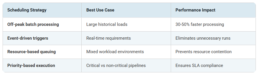
Scheduling ETL jobs reduces contention with operational systems. However, smart scheduling goes beyond simple timing:
Layers, contracts and canonical schema
A robust architecture is best described as layers governed by explicit contracts. At the perimeter, source connectors interact with APIs, brokers, file drops, and vendor feeds. Their contract is to emit raw events with source metadata, explicit time conventions, and enough information to reproduce the request.
Raw ingestion into OLTP should be append-heavy and minimally transformative. Its contract is to preserve raw information, enforce uniqueness, and preserve provenance. Canonicalization then converts heterogeneous source representations into a canonical schema by enforcing time normalization, type normalization, and symbol mapping. The DW layer provides partitioned fact tables and dimensions (assets, calendars, sources) with stable semantics optimized for analytical access.
Above the DW, a feature store publishes versioned feature vectors and tensors consumed by research and live engines. The feature store is the interface that enforces immutability by version and train/live parity. Finally, model inputs and backtest feeds are derived from the feature store as arrays, parquet datasets, or tight queries.
A canonical schema must minimize semantic ambiguity. At minimum, an asset dimension fixes identifiers, venues, tick sizes, and calendars. A calendar dimension fixes session definitions, holidays, and early closes. A source dimension fixes provider identity, endpoint sampling rules, time conventions, and revision policy. Facts separate raw events from derived bars and derived bars from derived features. This separation prevents circularity and leakage.
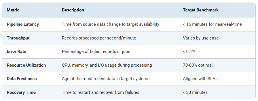
Establishing baseline metrics is essential before implementing optimization strategies. Track these KPIs to measure improvement:
A critical design choice is to represent bars with explicit start/end timestamps. Ambiguous labels are a recurring source of leakage.
CREATE TABLE IF NOT EXISTS fact_bar (
  asset_id           BIGINT NOT NULL,
  ts_start_utc       TIMESTAMPTZ NOT NULL,
  ts_end_utc         TIMESTAMPTZ NOT NULL,
  open               DOUBLE PRECISION,
  high               DOUBLE PRECISION,
  low                DOUBLE PRECISION,
  close              DOUBLE PRECISION,
  volume             DOUBLE PRECISION,
  source_id          TEXT NOT NULL,
  ingest_ts_utc      TIMESTAMPTZ NOT NULL DEFAULT NOW(),
  quality_flags      INTEGER NOT NULL DEFAULT 0,
  PRIMARY KEY (asset_id, ts_start_utc, source_id)
);

CREATE INDEX IF NOT EXISTS idx_fact_bar_end
  ON fact_bar(asset_id, ts_end_utc);
This schema forces a commitment to interval semantics and prevents a broad class of timestamp-induced lookahead errors.
CREATE TABLE IF NOT EXISTS feature_vector (
  asset_id            BIGINT NOT NULL,
  ts_utc              TIMESTAMPTZ NOT NULL,
  feature_set_version TEXT NOT NULL,
  f1                  DOUBLE PRECISION,
  f2                  DOUBLE PRECISION,
  f3                  DOUBLE PRECISION,
  quality_flags       INTEGER NOT NULL DEFAULT 0,
  PRIMARY KEY(asset_id, ts_utc, feature_set_version)
);
ETL vs ELT for trading
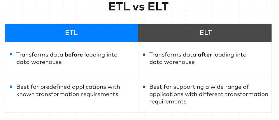
The distinction between ETL and ELT is often discussed in any development team, as if one pattern is better than the other. In trading, that framing is unhelpful because the decision is about which transformations are definitional—therefore part of the market representation—and which transformations are computational—therefore a choice of execution venue. A trading dataset is not data until its semantics are pinned down, and semantics are what many transformations decide.
The first class of transformations is semantic. These transformations determine what your system claims to observe and when. Time conventions are semantic because they define the filtration. If the vendor labels a bar by end time but you interpret it as start time, you have built a causal violation into your feature history. Calendars are semantic because they define what a day means (and therefore what daily VWAP, overnight gap, and close-to-open return mean). Instrument mapping is semantic because it defines what the identifier refers to under symbol changes, roll schedules, corporate actions, and contract specification updates. Definitional conformance is semantic because it defines what a field means: whether volume is shares, contracts, or notional; whether a price is last, mid, bid, or ask; whether OHLC is constructed from trades or quotes; and whether adjusted prices are being mixed with unadjusted prices. These transformations belong before the warehouse-facing analytical layer in the sense that they must be controlled, testable, and versioned as part of the dataset definition. Once you accept that, the ETL/ELT question becomes secondary: the definitional layer must exist, regardless of where the subsequent compute occurs.
The second class of transformations is computational. These transformations take an already-defined representation and compute derived quantities that don’t change the meaning of the underlying observables. Rolling sums, rolling standard deviations, exponentially weighted averages, joins across conformed facts, feature aggregation, and windowed statistics are computational. They can be done in the warehouse (ELT), in an external feature job (ETL in the broad sense), or in a feature store materialization step. If a computational feature is used across many models and many experiments, materializing it can be economically rational because it stabilizes definitions and reduces iteration latency.
A practical way to decide is to ask one question: does this transformation change the information boundary of the dataset? If it does, it must be treated as part of the dataset specification and therefore requires explicit contracts, deterministic behavior, and versioning. If it doesn’t, then the transformation is a compute-placement decision driven by throughput and operational constraints. This avoids a common failure mode where teams ELT everything.
For example, if we continue with the VWAP example, the decision to reset it at the boundary of an exchange trading day is semantic because it depends on the session calendar and therefore on a definition of day. The computation of VWAP itself—cumulative sums of price times volume divided by cumulative volume—is computational once the day boundary has been fixed. Similarly, defining what constitutes an overnight return is semantic because it depends on which close and which open are used (and whether the asset trades continuously). Computing the return itself is computational.
This is also why trading pipelines benefit from an explicit semantic conformance layer even when the team prefers ELT. In practice, this layer may live as a set of controlled SQL models, a dbt project, a set of stored procedures, or a Python conformance job that writes canonical facts—like the one below. The key is that semantic logic is centralized, versioned, and tested.
# SQLite
SQLITE_FACT_BAR_DDL = """
CREATE TABLE IF NOT EXISTS fact_bar (
  asset_id      INTEGER NOT NULL,
  ts_start_utc  TEXT NOT NULL,
  ts_end_utc    TEXT NOT NULL,
  open          REAL,
  high          REAL,
  low           REAL,
  close         REAL,
  volume        REAL,
  source_id     TEXT NOT NULL,
  ingest_ts_utc TEXT NOT NULL,
  quality_flags INTEGER NOT NULL DEFAULT 0,
  PRIMARY KEY (asset_id, ts_start_utc, source_id)
);
CREATE INDEX IF NOT EXISTS idx_fact_bar_end ON fact_bar(asset_id, ts_end_utc);
"""

SQLITE_FEATURE_VECTOR_DDL = """
CREATE TABLE IF NOT EXISTS feature_vector (
  asset_id            INTEGER NOT NULL,
  ts_utc              TEXT NOT NULL,
  feature_set_version TEXT NOT NULL,
  f1                  REAL,
  f2                  REAL,
  f3                  REAL,
  quality_flags       INTEGER NOT NULL DEFAULT 0,
  PRIMARY KEY(asset_id, ts_utc, feature_set_version)
);
"""

SQLITE_UPSERT_BAR_SQL = """
INSERT INTO fact_bar(asset_id, ts_start_utc, ts_end_utc, open, high, low, close, volume, source_id, ingest_ts_utc, quality_flags)
VALUES (?,?,?,?,?,?,?,?,?,?,?)
ON CONFLICT(asset_id, ts_start_utc, source_id)
DO UPDATE SET
  ts_end_utc    = excluded.ts_end_utc,
  open          = excluded.open,
  high          = excluded.high,
  low           = excluded.low,
  close         = excluded.close,
  volume        = excluded.volume,
  ingest_ts_utc = excluded.ingest_ts_utc,
  quality_flags = excluded.quality_flags;
"""

SQLITE_UPSERT_FEATURE_SQL = """
INSERT INTO feature_vector(asset_id, ts_utc, feature_set_version, f1, f2, f3, quality_flags)
VALUES (?,?,?,?,?,?,?)
ON CONFLICT(asset_id, ts_utc, feature_set_version)
DO UPDATE SET
  f1 = excluded.f1,
  f2 = excluded.f2,
  f3 = excluded.f3,
  quality_flags = excluded.quality_flags;
"""
A concise implementation pattern is to keep raw ingestion append-only and as close to source as possible, then apply a conformance step that pins down semantics, then perform computational features either in-warehouse or as a materialized feature job. In other words, a pragmatic hybrid is common: extract and load raw into OLTP with minimal mutation, transform into conformed DW tables, and materialize features into a versioned feature store. This preserves provenance while enabling analytical performance.
The ETL/ELT choice also interacts with latency and reliability. If you need intraday features with tight publication deadlines, pushing heavy joins and window functions into a shared warehouse can create contention and unpredictable runtimes. Conversely, if you compute everything outside the warehouse, you may replicate logic across scripts and drift into semantic inconsistency. A stable compromise is to push stable, high-fanout computations into materialized tables or feature store partitions, while keeping fragile semantics confined to a small, well-tested conformance layer.
To illustrate how semantic logic can remain explicit even in an ELT-heavy design, consider a canonical bar view that makes interval semantics and day identifiers visible to downstream consumers. The key idea is that the view should encode the definition, not only reshape columns.
CREATE OR REPLACE VIEW v_bar_canonical AS
SELECT
  asset_id,
  ts_start_utc,
  ts_end_utc,
  open, high, low, close,
  volume,
  source_id,
  date_trunc('day', ts_start_utc AT TIME ZONE 'UTC')::date AS day_id_utc,
  quality_flags
FROM fact_bar
WHERE ts_end_utc > ts_start_utc;
Once the semantics are fixed in canonical facts or views, computational features can be computed where it is most efficient. If you want the warehouse to own feature computation, you can materialize a feature table keyed by (asset_id, ts_utc, feature_set_version) and treat feature_set_version as a contract.
INSERT INTO feature_vector(asset_id, ts_utc, feature_set_version, f1, f2, f3, quality_flags)
SELECT
  asset_id,
  ts_end_utc AS ts_utc,
  '1.0.0' AS feature_set_version,
  ln(close) - ln(lag(close) OVER w) AS f1,
  close - (sum(close * volume) OVER wd) / NULLIF(sum(volume) OVER wd, 0) AS f2,
  stddev_samp(ln(close) - ln(lag(close) OVER w)) OVER w20 AS f3,
  max(quality_flags) OVER w AS quality_flags
FROM v_bar_canonical
WINDOW
  w  AS (PARTITION BY asset_id ORDER BY ts_end_utc),
  w20 AS (PARTITION BY asset_id ORDER BY ts_end_utc ROWS BETWEEN 19 PRECEDING AND CURRENT ROW),
  wd AS (PARTITION BY asset_id, day_id_utc ORDER BY ts_end_utc);
The goal of these snippets is to show that the definitional layer can remain explicit, inspectable, and testable even when feature computation is executed inside the warehouse. If, instead, you prefer external feature jobs, the same contract still applies.

What breaks ETL in trading systems
Heterogeneity and conformance are the first obstacles because they are structural. A conformance layer must normalize identifiers, time bases, session calendars, field semantics, and types. To make this enforceable, treat conformance as a mapping between typed domains. A source-level record belongs to a source domain Xs, and conformance maps it to a canonical domain X* via Φs: Xs →X*. If Φs changes, you have changed the dataset, even if downstream schemas remain identical.
Missing data is structural. For backtesting, NaN propagation is often preferable to imputation because it preserves ignorance. For live systems, “don’t crash” constraints exist, but fallbacks must be conservative: don’t invent OHLC; carry forward last observed values only for risk checks, not alpha computation; set quality flags; and disable signal generation for assets that violate completeness constraints. A useful principle is that a live fallback should minimize the probability of trading on corrupted information, even at the cost of missed trades.
API limits and latency budgets impose feasibility constraints. If the provider caps calls per minute and each call has a nontrivial wall time, there is a hard bound on how much data can be collected and published per day. If those bounds are violated, no amount of clever modelling will compensate; the design must change via batching, parallelization under caps, endpoint scope reduction, or provider selection.
Performance pathologies arise when feature computation is with conformance and aggregation. Recomputing features inside model selection loops expands iteration time and changes which hypotheses you can afford to test. Materialization reduces repeated computation, but it also increases the importance of versioning. A pipeline must separate semantic conformance, structural aggregation, computational feature construction, and statistical modelling.
Schema drift includes semantic drift: fields retain names while changing meaning. Without a schema/semantic registry, and without semantic versioning of transformations, a pipeline can mutate what the data means. Security and access control are baseline requirements because trading pipelines store proprietary features and operational metadata.
The following plan is minimalist and is designed as an example. In the appendix, I’ve included another, a little bit more detailed.
Extraction requires deterministic request generation, rate-limit aware scheduling, retries with backoff, and optional raw-response archiving for forensic analysis.
import time
import json
import random
from urllib.request import urlopen, Request

class RateLimiter:
    def __init__(self, max_per_minute: int):
        self.max_per_minute = int(max_per_minute)
        self.min_interval = 60.0 / float(self.max_per_minute)
        self._t_last = 0.0

    def wait(self):
        dt = time.time() - self._t_last
        if dt < self.min_interval:
            time.sleep(self.min_interval - dt)
        self._t_last = time.time()


def fetch_json(url: str, limiter: RateLimiter, max_retries: int = 5) -> dict:
    for attempt in range(max_retries):
        try:
            limiter.wait()
            req = Request(url, headers={"User-Agent": "quant-etl/1.0"})
            with urlopen(req, timeout=20) as r:
                return json.loads(r.read().decode("utf-8"))
        except Exception:
            sleep_s = (2 ** attempt) + random.random()
            time.sleep(sleep_s)
    raise RuntimeError(f"Failed to fetch after {max_retries} retries: {url}")
Transformation should be expressed as pure functions: normalize timestamps into UTC with explicit interval semantics, normalize numeric types, and attach quality metadata.
from datetime import datetime, timezone, timedelta

def to_utc(ts_str: str) -> datetime:
    dt = datetime.fromisoformat(ts_str.replace("Z", "+00:00"))
    return dt.astimezone(timezone.utc)


def conform_bar(raw: dict, asset_id: int, source_id: str, bar_minutes: int) -> Bar:
    ts_end = to_utc(raw["date"])  # interpret explicitly as bar end
    ts_start = ts_end - timedelta(minutes=int(bar_minutes))

    open_  = float(raw.get("open", "nan"))
    high_  = float(raw.get("high", "nan"))
    low_   = float(raw.get("low",  "nan"))
    close_ = float(raw.get("close","nan"))
    vol_   = float(raw.get("volume","nan"))

    return Bar(
        asset_id=asset_id,
        ts_start_utc=ts_start,
        ts_end_utc=ts_end,
        open=open_, high=high_, low=low_, close=close_, volume=vol_,
        source_id=source_id,
    )
Loading should be batched and idempotent. Batching is an engineering constraint, idempotence is an epistemic constraint.
def chunked(iterable, size: int):
    buf = []
    for x in iterable:
        buf.append(x)
        if len(buf) >= size:
            yield buf
            buf = []
    if buf:
        yield buf
Finally, a quality gate must exist. If QC flags exceed thresholds, the system may still ingest and store raw data, but it shouldn’t publish features to the live engine. This is the smallest mechanism that prevents a strategy from trading on corrupted representations.
Let’s see what this example can offer us!
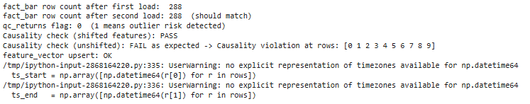

Okay! Basically what was expected.

Alright crew—solid session. Until the next bell: keep your process boring, your sizing honest, and your rules louder than your mood. May liquidity show up when you need it, slippage stay polite, and your cleanest edges stack quietly while the crowd chases noise 💵
PS: What is more important for you?
This is an invitation-only access to our QUANT COMMUNITY, so we verify numbers to avoid spammers and scammers. Feel free to join or decline at any time. Tap the WhatsApp icon below to join

Appendix
Full script for an ETL
import time
import json
import random
import hashlib
import sqlite3
from dataclasses import dataclass
from datetime import datetime, timezone, timedelta
from urllib.request import urlopen, Request
import numpy as np
import matplotlib.pyplot as plt
# QL schemas
POSTGRES_FACT_BAR_DDL = r"""
-- PostgreSQL-style DDL (conceptually portable)
CREATE TABLE IF NOT EXISTS fact_bar (
asset_id BIGINT NOT NULL,
ts_start_utc TIMESTAMPTZ NOT NULL,
ts_end_utc TIMESTAMPTZ NOT NULL,
open DOUBLE PRECISION,
high DOUBLE PRECISION,
low DOUBLE PRECISION,
close DOUBLE PRECISION,
volume DOUBLE PRECISION,
source_id TEXT NOT NULL,
ingest_ts_utc TIMESTAMPTZ NOT NULL DEFAULT NOW(),
quality_flags INTEGER NOT NULL DEFAULT 0,
PRIMARY KEY (asset_id, ts_start_utc, source_id)
);
CREATE INDEX IF NOT EXISTS idx_fact_bar_end
ON fact_bar(asset_id, ts_end_utc);
"""
POSTGRES_FEATURE_VECTOR_DDL = r"""
CREATE TABLE IF NOT EXISTS feature_vector (
asset_id BIGINT NOT NULL,
ts_utc TIMESTAMPTZ NOT NULL,
feature_set_version TEXT NOT NULL,
f1 DOUBLE PRECISION,
f2 DOUBLE PRECISION,
f3 DOUBLE PRECISION,
quality_flags INTEGER NOT NULL DEFAULT 0,
PRIMARY KEY(asset_id, ts_utc, feature_set_version)
);
"""
POSTGRES_UPSERT_BAR_SQL = r"""
INSERT INTO fact_bar(asset_id, ts_start_utc, ts_end_utc, open, high, low, close, volume, source_id, quality_flags)
VALUES ($1,$2,$3,$4,$5,$6,$7,$8,$9,$10)
ON CONFLICT (asset_id, ts_start_utc, source_id)
DO UPDATE SET
ts_end_utc = EXCLUDED.ts_end_utc,
open = EXCLUDED.open,
high = EXCLUDED.high,
low = EXCLUDED.low,
close = EXCLUDED.close,
volume = EXCLUDED.volume,
quality_flags = EXCLUDED.quality_flags;
"""
# SQLite
SQLITE_FACT_BAR_DDL = """
CREATE TABLE IF NOT EXISTS fact_bar (
asset_id INTEGER NOT NULL,
ts_start_utc TEXT NOT NULL,
ts_end_utc TEXT NOT NULL,
open REAL,
high REAL,
low REAL,
close REAL,
volume REAL,
source_id TEXT NOT NULL,
ingest_ts_utc TEXT NOT NULL,
quality_flags INTEGER NOT NULL DEFAULT 0,
PRIMARY KEY (asset_id, ts_start_utc, source_id)
);
CREATE INDEX IF NOT EXISTS idx_fact_bar_end ON fact_bar(asset_id, ts_end_utc);
"""
SQLITE_FEATURE_VECTOR_DDL = """
CREATE TABLE IF NOT EXISTS feature_vector (
asset_id INTEGER NOT NULL,
ts_utc TEXT NOT NULL,
feature_set_version TEXT NOT NULL,
f1 REAL,
f2 REAL,
f3 REAL,
quality_flags INTEGER NOT NULL DEFAULT 0,
PRIMARY KEY(asset_id, ts_utc, feature_set_version)
);
"""
SQLITE_UPSERT_BAR_SQL = """
INSERT INTO fact_bar(asset_id, ts_start_utc, ts_end_utc, open, high, low, close, volume, source_id, ingest_ts_utc, quality_flags)
VALUES (?,?,?,?,?,?,?,?,?,?,?)
ON CONFLICT(asset_id, ts_start_utc, source_id)
DO UPDATE SET
ts_end_utc = excluded.ts_end_utc,
open = excluded.open,
high = excluded.high,
low = excluded.low,
close = excluded.close,
volume = excluded.volume,
ingest_ts_utc = excluded.ingest_ts_utc,
quality_flags = excluded.quality_flags;
"""
SQLITE_UPSERT_FEATURE_SQL = """
INSERT INTO feature_vector(asset_id, ts_utc, feature_set_version, f1, f2, f3, quality_flags)
VALUES (?,?,?,?,?,?,?)
ON CONFLICT(asset_id, ts_utc, feature_set_version)
DO UPDATE SET
f1 = excluded.f1,
f2 = excluded.f2,
f3 = excluded.f3,
quality_flags = excluded.quality_flags;
"""
# YAML
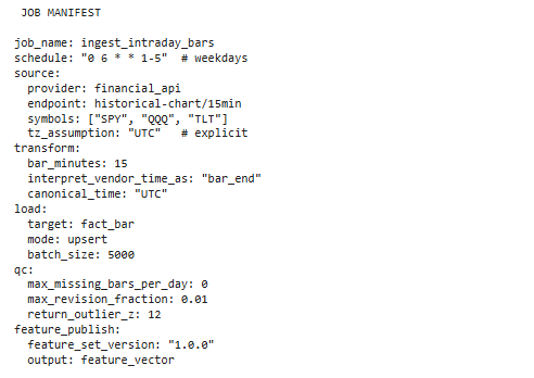
JOB_MANIFEST_YAML = r"""
job_name: ingest_intraday_bars
schedule: "0 6 * * 1-5" # weekdays
source:
provider: financial_api
endpoint: historical-chart/15min
symbols: ["SPY", "QQQ", "TLT"]
tz_assumption: "UTC" # explicit
transform:
bar_minutes: 15
interpret_vendor_time_as: "bar_end"
canonical_time: "UTC"
load:
target: fact_bar
mode: upsert
batch_size: 5000
qc:
max_missing_bars_per_day: 0
max_revision_fraction: 0.01
return_outlier_z: 12
feature_publish:
feature_set_version: "1.0.0"
output: feature_vector
"""
# RateLimiter + fetch_json
class RateLimiter:
def __init__(self, max_per_minute: int):
self.max_per_minute = int(max_per_minute)
self.min_interval = 60.0 / float(self.max_per_minute)
self._t_last = 0.0
def wait(self):
dt = time.time() - self._t_last
if dt < self.min_interval:
time.sleep(self.min_interval - dt)
self._t_last = time.time()
def fetch_json(url: str, limiter: RateLimiter, max_retries: int = 5) -> dict:
for attempt in range(max_retries):
try:
limiter.wait()
req = Request(url, headers={"User-Agent": "quant-etl/1.0"})
with urlopen(req, timeout=20) as r:
return json.loads(r.read().decode("utf-8"))
except Exception:
sleep_s = (2 ** attempt) + random.random()
time.sleep(sleep_s)
raise RuntimeError(f"Failed to fetch after {max_retries} retries: {url}")
# Bar dataclass + hash
@dataclass(frozen=True)
class Bar:
asset_id: int
ts_start_utc: datetime
ts_end_utc: datetime
open: float
high: float
low: float
close: float
volume: float
source_id: str
def natural_key(self) -> tuple:
return (self.asset_id, self.ts_start_utc, self.source_id)
def payload_hash(self) -> str:
s = (
f"{self.asset_id}|{self.ts_start_utc.isoformat()}|{self.ts_end_utc.isoformat()}|"
f"{self.open}|{self.high}|{self.low}|{self.close}|{self.volume}|{self.source_id}"
)
return hashlib.sha256(s.encode("utf-8")).hexdigest()
#Transform helpers
def to_utc(ts_str: str) -> datetime:
dt = datetime.fromisoformat(ts_str.replace("Z", "+00:00"))
return dt.astimezone(timezone.utc)
def conform_bar(raw: dict, asset_id: int, source_id: str, bar_minutes: int) -> Bar:
ts_end = to_utc(raw["date"]) # interpret explicitly as bar end
ts_start = ts_end - timedelta(minutes=int(bar_minutes))
open_ = float(raw.get("open", "nan"))
high_ = float(raw.get("high", "nan"))
low_ = float(raw.get("low", "nan"))
close_ = float(raw.get("close","nan"))
vol_ = float(raw.get("volume","nan"))
return Bar(
asset_id=asset_id,
ts_start_utc=ts_start,
ts_end_utc=ts_end,
open=open_, high=high_, low=low_, close=close_, volume=vol_,
source_id=source_id,
)
def chunked(iterable, size: int):
buf = []
for x in iterable:
buf.append(x)
if len(buf) >= size:
yield buf
buf = []
if buf:
yield buf
# Causality assertion
def assert_causal_features(feature_ts_end_utc: np.ndarray, decision_ts_utc: np.ndarray):
if np.any(decision_ts_utc < feature_ts_end_utc):
bad = np.where(decision_ts_utc < feature_ts_end_utc)[0][:10]
raise AssertionError(f"Causality violation at rows: {bad}")
# QC returns (robust z using MAD)
def qc_returns(close: np.ndarray, z_thresh: float = 12.0) -> int:
close = np.asarray(close, dtype=np.float64)
r = np.diff(np.log(close))
med = np.nanmedian(r)
mad = np.nanmedian(np.abs(r - med))
if (not np.isfinite(mad)) or mad == 0.0:
return 1
z = (r - med) / (1.4826 * mad)
return int(np.nanmax(np.abs(z)) > float(z_thresh))
# Feature pipeline (daily VWAP reset + rolling std)
def daily_reset_vwap(price: np.ndarray, vol: np.ndarray, day_id: np.ndarray) -> np.ndarray:
price = np.asarray(price, dtype=np.float64)
vol = np.asarray(vol, dtype=np.float64)
day_id = np.asarray(day_id)
out = np.empty_like(price, dtype=np.float64)
pv = price * vol
boundaries = np.flatnonzero(np.r_[True, day_id[1:] != day_id[:-1]])
boundaries = np.r_[boundaries, len(day_id)]
for s, e in zip(boundaries[:-1], boundaries[1:]):
cum_pv = np.cumsum(pv[s:e])
cum_v = np.cumsum(vol[s:e])
out[s:e] = np.where(cum_v > 0.0, cum_pv / cum_v, np.nan)
return out
def rolling_std(x: np.ndarray, w: int) -> np.ndarray:
x = np.asarray(x, dtype=np.float64)
out = np.full_like(x, np.nan)
w = int(w)
if w < 2:
return out
for i in range(w - 1, len(x)):
seg = x[i - w + 1:i + 1]
out[i] = np.nanstd(seg, ddof=1)
return out
def compute_features(close: np.ndarray, vol: np.ndarray, day_id: np.ndarray, w_vol: int = 20):
close = np.asarray(close, dtype=np.float64)
vol = np.asarray(vol, dtype=np.float64)
r = np.empty_like(close)
r[0] = np.nan
r[1:] = np.diff(np.log(close))
vwap = daily_reset_vwap(close, vol, day_id)
sig = rolling_std(r, w=w_vol)
X = np.column_stack([r, close - vwap, sig])
return X
# DB layer (SQLite) - idempotent upsert + reads
def init_db(conn: sqlite3.Connection):
cur = conn.cursor()
cur.executescript(SQLITE_FACT_BAR_DDL)
cur.executescript(SQLITE_FEATURE_VECTOR_DDL)
conn.commit()
def upsert_bars(conn: sqlite3.Connection, bars: list[Bar], quality_flags: int = 0, batch_size: int = 5000):
cur = conn.cursor()
ingest_now = datetime.now(timezone.utc).isoformat()
rows = []
for b in bars:
rows.append((
int(b.asset_id),
b.ts_start_utc.isoformat(),
b.ts_end_utc.isoformat(),
float(b.open), float(b.high), float(b.low), float(b.close), float(b.volume),
str(b.source_id),
ingest_now,
int(quality_flags),
))
for chunk in chunked(rows, batch_size):
cur.executemany(SQLITE_UPSERT_BAR_SQL, chunk)
conn.commit()
def count_fact_bars(conn: sqlite3.Connection) -> int:
cur = conn.cursor()
cur.execute("SELECT COUNT(*) FROM fact_bar;")
return int(cur.fetchone()[0])
def load_bars_arrays(conn: sqlite3.Connection, asset_id: int, source_id: str):
cur = conn.cursor()
cur.execute(
"""
SELECT ts_start_utc, ts_end_utc, open, high, low, close, volume, quality_flags
FROM fact_bar
WHERE asset_id = ? AND source_id = ?
ORDER BY ts_start_utc ASC;
""",
(int(asset_id), str(source_id)),
)
rows = cur.fetchall()
if not rows:
raise RuntimeError("No bars found.")
ts_start = np.array([np.datetime64(r[0]) for r in rows])
ts_end = np.array([np.datetime64(r[1]) for r in rows])
open_ = np.array([r[2] for r in rows], dtype=np.float64)
high_ = np.array([r[3] for r in rows], dtype=np.float64)
low_ = np.array([r[4] for r in rows], dtype=np.float64)
close_ = np.array([r[5] for r in rows], dtype=np.float64)
vol_ = np.array([r[6] for r in rows], dtype=np.float64)
qf = np.array([r[7] for r in rows], dtype=np.int64)
return ts_start, ts_end, open_, high_, low_, close_, vol_, qf
def upsert_feature_vectors(conn: sqlite3.Connection,
asset_id: int,
ts_utc: np.ndarray,
X: np.ndarray,
feature_set_version: str,
quality_flags: int = 0,
batch_size: int = 5000):
ts_utc = np.asarray(ts_utc)
X = np.asarray(X, dtype=np.float64)
if X.ndim != 2 or X.shape[1] < 3:
raise ValueError("X must be (n,>=3) for f1,f2,f3.")
cur = conn.cursor()
rows = []
for i in range(len(ts_utc)):
# store ISO string
ts_s = str(ts_utc[i]).replace(" ", "T")
rows.append((int(asset_id), ts_s, str(feature_set_version),
float(X[i, 0]), float(X[i, 1]), float(X[i, 2]),
int(quality_flags)))
for chunk in chunked(rows, batch_size):
cur.executemany(SQLITE_UPSERT_FEATURE_SQL, chunk)
conn.commit()
# Make synthetic "raw API" bars
def make_synthetic_raw_bars(start_end_utc: datetime,
n_bars: int,
bar_minutes: int = 15,
seed: int = 7):
"""
Produces raw bars where "date" is the *bar end* timestamp in ISO Z (like many vendors).
"""
rng = np.random.default_rng(seed)
out = []
# price random walk
price = 100.0
dt = timedelta(minutes=int(bar_minutes))
ts_end = start_end_utc
for _ in range(n_bars):
# simulate end-to-end bar
ret = rng.normal(0.0, 0.001) # small drift/noise
close = price * np.exp(ret)
high = max(price, close) * (1.0 + abs(rng.normal(0.0, 0.0007)))
low = min(price, close) * (1.0 - abs(rng.normal(0.0, 0.0007)))
open_ = price
vol = float(max(1.0, rng.lognormal(mean=4.5, sigma=0.4))) # positive
out.append({
"date": ts_end.isoformat().replace("+00:00", "Z"),
"open": open_,
"high": high,
"low": low,
"close": close,
"volume": vol,
})
price = close
ts_end = ts_end + dt
return out
def day_id_from_ts_end(ts_end: np.ndarray) -> np.ndarray:
# day_id = YYYYMMDD integer using ts_end UTC date
days = np.array([str(t)[:10].replace("-", "") for t in ts_end], dtype=np.int64)
return days
# ETL + QC + Features + Causality test + plot
def main():
# demo config
asset_id = 1
source_id = "demo_vendor"
bar_minutes = 15
feature_set_version = "1.0.0"
w_vol = 20
# (1) EXTRACT (synthetic)
start_end_utc = datetime(2026, 2, 2, 0, 0, tzinfo=timezone.utc)
n_bars = 3 * 24 * (60 // bar_minutes) # 3 days of 15-min bars
raw = make_synthetic_raw_bars(start_end_utc=start_end_utc, n_bars=n_bars, bar_minutes=bar_minutes)
# (2) TRANSFORM (conform)
bars = [conform_bar(r, asset_id=asset_id, source_id=source_id, bar_minutes=bar_minutes) for r in raw]
# (3) LOAD (idempotent upsert)
conn = sqlite3.connect(":memory:")
init_db(conn)
upsert_bars(conn, bars, quality_flags=0, batch_size=5000)
n1 = count_fact_bars(conn)
# rerun same load to prove idempotence
upsert_bars(conn, bars, quality_flags=0, batch_size=5000)
n2 = count_fact_bars(conn)
print(f"fact_bar row count after first load: {n1}")
print(f"fact_bar row count after second load: {n2} (should match)")
# read back as arrays
ts_start, ts_end, open_, high_, low_, close_, vol_, qf = load_bars_arrays(conn, asset_id, source_id)
day_id = day_id_from_ts_end(ts_end)
# QC (dataset-level flag, minimal demo)
qc_flag = qc_returns(close_, z_thresh=12.0)
print(f"qc_returns flag: {qc_flag} (1 means outlier risk detected)")
# FEATURES (train/live parity rule for bar-open execution)
# compute features using series as-given (bars labeled by end-time)
X_raw = compute_features(close_, vol_, day_id, w_vol=w_vol)
# For bar-open decisions at ts_start[k], enforce "only info strictly before that open":
# shift features by 1 bar so X_used[k] depends on bars ending <= ts_start[k].
X_used = np.empty_like(X_raw)
X_used[:] = np.nan
X_used[1:] = X_raw[:-1]
# causality timestamps: feature window "ends" at previous bar end (ts_end[k-1])
feature_ts_end = np.empty_like(ts_end)
feature_ts_end[:] = np.datetime64("NaT")
feature_ts_end[1:] = ts_end[:-1]
decision_ts = ts_start.copy()
# causality test (should pass)
assert_causal_features(feature_ts_end, decision_ts)
print("Causality check (shifted features): PASS")
# demonstrate failure if you (incorrectly) use current bar end as if available at open
try:
assert_causal_features(ts_end, decision_ts) # BAD: decision at start < end
print("Causality check (unshifted): PASS (unexpected)")
except AssertionError as e:
print(f"Causality check (unshifted): FAIL as expected -> {e}")
# (5) PUBLISH features into feature store table
upsert_feature_vectors(
conn,
asset_id=asset_id,
ts_utc=decision_ts, # label features at decision time
X=X_used,
feature_set_version=feature_set_version,
quality_flags=qc_flag,
)
print("feature_vector upsert: OK")
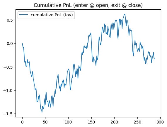
# (6) Tiny example signal + PnL (just to validate arrays end-to-end)
# mean-reversion toy: if close - vwap > 0 => short, else long; 0 when NaN
f2 = X_used[:, 1]
sig = np.where(np.isfinite(f2), np.where(f2 > 0.0, -1.0, 1.0), 0.0)
# bar PnL if entering at open and exiting at close of same bar
pnl = sig * (close_ - open_)
pnl_cum = np.nancumsum(np.where(np.isfinite(pnl), pnl, 0.0))
# Plot 1: close vs VWAP (from X_raw, because VWAP exists at bar end)
vwap_end = close_ - X_raw[:, 1]
plt.figure()
plt.plot(close_, label="close")
plt.plot(vwap_end, label="vwap (daily reset)")
plt.title("Close vs Daily-Reset VWAP (computed at bar end)")
plt.legend()
plt.show()
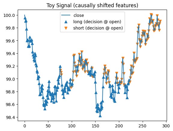
# Plot 2: decision-time signal markers on close (using shifted features)
plt.figure()
plt.plot(close_, label="close")
idx_long = np.where(sig == 1.0)[0]
idx_short = np.where(sig == -1.0)[0]
plt.scatter(idx_long, close_[idx_long], marker="^", label="long (decision @ open)")
plt.scatter(idx_short, close_[idx_short], marker="v", label="short (decision @ open)")
plt.title("Toy Signal (causally shifted features)")
plt.legend()
plt.show()
# Plot 3: cumulative PnL (toy)
plt.figure()
plt.plot(pnl_cum, label="cumulative PnL (toy)")
plt.title("Cumulative PnL (enter @ open, exit @ close)")
plt.legend()
plt.show()
print("\n JOB MANIFEST")
print(JOB_MANIFEST_YAML)
main()