[WITH CODE] Switch-off: Conformal-RANSAC kill switch

Conformal Prediction coupled with RANSAC to switch-off portfolios

---

Table of contents:

1. Introduction.

2. The trend validation trap.

3. Risk and model limitations.

4. What are the obstacles to face when developing this kind of algorithms?

5. Theoretical foundation.

   1. Point 1: The linear necessity and the failure of OLS.

   2. Point 2: The RANSAC algorithm construction.

   3. Point 3: The split-Conformal Prediction framework.

   4. Point 4: The strict positivity logic

6. Operationalization.

   1. Engineering the Conformal-RANSAC.

---

Introduction

In systematic portfolio management, the question that matters isn’t whether a strategy has been profitable in a backtest or over a recent window—it’s whether the process generating that profit still deserves capital right now. Industry practice tends to compress that decision into a single, comforting statistic: fit a straight line to the equity curve and ask whether the estimated slope is positive with enough confidence. On paper, this is clean. In production, it is dangerously brittle. A PnL curve is not a textbook signal but an object shaped by microstructure effects, intermittent liquidity, and rare events that are not rare enough. Under those conditions, the usual regression tools don’t merely lose precision—they can invert the meaning of evidence, mistaking a single lucky outlier for a restored edge or treating a brief but violent drawdown as proof of structural decay.

This is the trend validation trap: we want a kill-switch that enforces a strict positivity constraint on performance, because capital should not sit inside a system that is not demonstrably compounding. Yet the standard method used to measure trend is built on squared-error minimization, which amplifies precisely the observations we should distrust most. The consequence is a conflict between operational necessity and statistical fragility. If we keep the rule but rely on OLS, we risk zombie strategies surviving on the back of one exceptional trade, and healthy strategies getting shut down due to a transient tail event or a bad print. If we abandon the rule, we drift back into discretionary tolerance bands and post-hoc rationalizations—exactly the failure mode a kill-switch is meant to prevent.

The framework developed here resolves that conflict by reframing the problem from “fit the data” to “validate the structure.” It is based on several papers that you can find here:

Conformalize Quantile Regression

1.36MB ∙ PDF file

Download

Download

Adaptive Conformal Inference

825KB ∙ PDF file

Download

Download

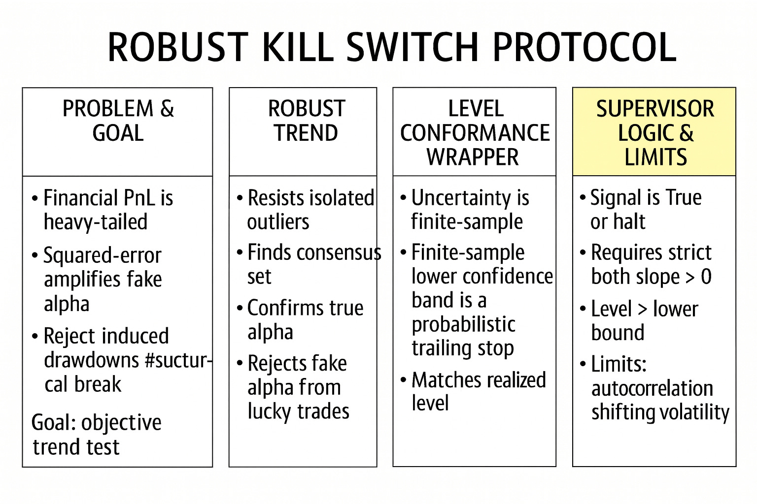
First, we replace the regression objective with a robustness principle: RANSAC searches for the dominant linear drift supported by the majority of observations and treats the tails as contamination rather than evidence. Second, we move from asymptotic confidence language to finite-sample guarantees by calibrating uncertainty with split conformal prediction, producing a dynamic lower bound that behaves like a probabilistic trailing stop. Finally, we weld these components into a strict logic gate: capital is allocated only if the robust drift is positive and current performance remains inside a statistically valid corridor around that drift. The result is not a prettier line through the equity curve; it is a geometric protocol for deciding when a strategy has earned the right to continue trading, and when the burden of proof has not been met.

The trend validation trap

In quantitative portfolio management, the most fundamental question we ask of any active strategy is deceptively simple:

Is it working?

Operationally, this translates to a statistical hypothesis test:

Is the PnL trend strictly positive with high statistical confidence?

The initial dilemma is the trend validation trap. In the industry, we typically answer this question using Ordinary Least Squares (OLS) regression on the equity curve. We fit a linear model

\(y_t = \beta t + \alpha + \epsilon_t\)

and check if the slope coefficient β is positive. However, OLS is notoriously fragile in the context of financial time series. It operates by minimizing the sum of squared residuals. This quadratic loss function grants disproportionate influence to outliers—observations that lie far from the mean trend.

A single large outlier—a lucky trade driven by an exogenous liquidity event or a data artifact—can act as a high-leverage point, skewing the regression slope β significantly upwards. A strategy might exhibit a positive OLS slope solely due to one massive outlier, while bleeding capital on 95% of its trades (negative median PnL). Conversely, a healthy strategy might show a negative OLS slope during a short, sharp drawdown that is merely noise within a heavy-tailed distribution.

We face a critical conflict: we need a kill-switch that enforces a strict positivity constraint on the PnL trend, effectively demanding that the strategy demonstrates consistent alpha generation. Yet, we cannot rely on standard regression tools to measure that trend because they conflate variance with structural performance. The dilemma is how to distinguish between a strategy that is truly broken (structural decay of edge) and one that is merely suffering from heavy-tailed noise, without succumbing to the non-robustness of squared-error minimization.

Risk and model limitations

To solve this, we introduce a robust approach: Conformal Prediction coupled with RANSAC (Random Sample Consensus) Regression.

What is RANSAC?

RANSAC fundamentally inverts the philosophy of regression. While OLS attempts to model the entire dataset by minimizing average error, RANSAC assumes the dataset is a mixture of two distinct generating processes: “inliers” (the true signal/trend) and “outliers” (noise that should be ignored). It does not fit the data; it finds the data that fits the model.

It operates via an iterative hypothesize-and-verify loop:

1. Hypothesize: The algorithm randomly selects a minimal subset of data points (e.g., just two points) to analytically define a candidate linear model.

2. Verify: It tests this candidate trend against the entire dataset. It counts how many points fall within a strict tolerance band ±δ of the candidate line. These points form the Consensus Set.

3. Optimize: It repeats this process hundreds or thousands of times, ultimately selecting the model that maximizes the cardinality of the Consensus Set (i.e., the line that explains the largest number of trades).

In the context of a PnL curve, RANSAC effectively asks: “Is there a consistent, positive slope that explains the majority of the trades, if we ignore the shock events?” This makes it a lie detector for “fake alpha”—it rejects positive trends driven solely by outliers because those outliers will not form a large enough consensus set to validate the slope.

However, implementing this in production introduces specific operational and statistical risks:

1. The inlier bias and regime aliasing
   RANSAC works by finding the subset of data that fits a linear model best. In a trading context, there is a risk that the algorithm identifies a healthy subset of trades as inliers and dismisses the losses as outliers. This is regime aliasing. If a strategy is losing money consistently but has a few winning streaks, RANSAC might latch onto the winning streaks as the true trend and ignore the catastrophic losses as noise, provided the winning streaks are linear and numerous enough. The definition of the residual_threshold becomes the arbiter of reality; set it too tight, and the model overfits to noise; set it too loose, and it accepts broken trends.

2. The conformal coverage gap
   We use split Conformal Prediction to build a dynamic lower bound (a trailing stop based on probability). We calibrate a quantile q such that P(Y_new∈Ĉ) ≥ 1-α. This provides finite-sample validity, unlike asymptotic confidence intervals. However, the risk lies in the exchangeability assumption. Conformal prediction guarantees coverage only if the calibration residuals are exchangeable with the test residuals. In finance, volatility clustering violates this. A kill-switch calibrated during a low-volatility regime might fail to cover the residuals during a volatility explosion, triggering a false kill signal just when the strategy needs breathing room. The calibration window must be representative of the current volatility regime, or the coverage guarantee collapses.

3. The lope-level conflict
   Our proposed kill-switch logic uses a dual condition that establishes a hierarchy of failure:

   1. Slope condition: The robust trend must be positive (β_RANSAC> 0). This ensures the strategy is generating alpha directionally.

   2. Level condition: The current PnL must be above the conformal lower bound (PnL_t > ŷ_t - q). This ensures the strategy has not realized a drawdown that is statistically improbable given its valid trend.

   This creates a conflict in turnaround scenarios. A strategy can have a positive slope (recovering vigorously) but still be below the lower bound (deep in a drawdown hole). Conversely, it can be above the lower bound (shallow drawdown) but have a negative slope (beginning to rot). The risk involves defining the operational precedence: do we kill a strategy that is recovering but statistically too low, or do we keep a strategy that is high but statistically rotting? The model defaults to kill if either fails, which is a conservative, capital-preservation stance.

If you want to go deeper into Conformal Prediction, check out this Quant Lecture:

[Quant Lecture] Distribution Free

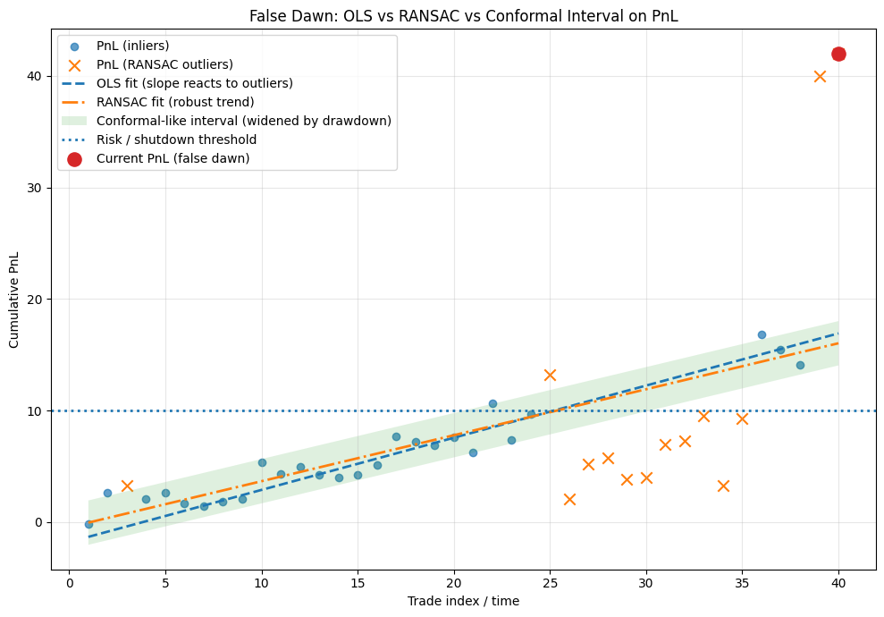
The core risk crystallizes during a false Dawn. Imagine a Momentum strategy that has suffered a significant 10% drawdown over two months. Suddenly, it prints a series of highly profitable trades due to a short-term volatility spike or a favorable macro announcement.

An OLS regression would immediately react to these large positive values, flipping the slope β from negative to positive, signaling “all clear.” A trader looking at the raw PnL would see a sharp uptick and feel relief. However, the RANSAC algorithm, robust to outliers, might reject these new profits as anomalies if they don’t fit the dominant (negative) trend established by the majority of trades in the window. To RANSAC, this is just high-magnitude noise, not a structural return to form.

Simultaneously, the Conformal interval, widened by the recent volatility of the drawdown, might still position the current PnL below the critical threshold defined by the calibration set. The pivotal event is this disagreement: The trader sees profits; the model sees noise. The decision to halt trading here is painful but necessary if we adhere to the philosophy that only robust trends constitute valid alpha. We need a mechanism that enforces this by rejecting the false dawn until the structure of the PnL proves it has healed, preventing re-entry into a strategy that is merely thrashing before failing completely.

What are the obstacles to face when developing this kind of algorithms?

The challenge is to construct a robust envelope around our PnL. We are moving away from simple lines in the sand (e.g., “stop at -$10k” or “stop at -15% MDD”) towards a dynamic, probabilistic tunnel that adapts to the strategy’s behavior.

We treat the PnL curve not as a deterministic financial accounting record, but as a noisy signal emitted by a stochastic physical process. Our goal is to extract the trajectory of the true process (via RANSAC) and bound its uncertainty (via Conformal Prediction). This shifts the burden of proof:

The strategy is assumed to be broken (signal False) unless it can prove it has a positive robust slope and is performing within its probabilistic bounds. The envelope acts as a dynamic hypothesis test performed at every time step, validating both the direction (slope) and the magnitude (level) of the performance.

In this terms there are 3 main obstacles we need to overcome:

1. The RANSAC stochasticity:
   RANSAC is intrinsically non-deterministic. It relies on random sub-sampling to find the best fit. In a production environment, running the same check twice on the same data could theoretically yield different results (kill vs. keep) if the max_trials parameter is too low or the data is highly ambiguous (low signal-to-noise ratio). We face the obstacle of stabilizing a randomized algorithm for a deterministic decision process. This requires setting of the random seed and ensuring max_trials is sufficient to reach a 99.99% probability of finding the optimal consensus set.

2. The calibration window dilemma:
   How much history do we feed the model? The length of the calibration window determines the memory of the volatility estimate. If we use min_history=50 trades, the conformal bounds are jumpy and loose, reacting wildly to recent volatility. If we use min_history=500, the bounds are tight but the model has massive inertia—it will be slow to react to a sudden strategy decay. Balancing the responsiveness of the RANSAC fit with the stability of the Conformal calibration is the central tuning challenge. We must find a window size that captures the relevant regime without introducing excessive lag.

3. The strict positivity constraint:
   The logic requires line_positive = (slope > 0) AND (trend_prediction > 0). This is a harsh constraint. A flat strategy (β≈0) is treated the same as a losing strategy. In a zero-interest-rate environment, holding a flat strategy might be acceptable. In a high-opportunity-cost environment, it is unacceptable. The obstacle is cultural: convincing stakeholders that a flat strategy is a broken strategy because it consumes capital, risk budget, and operational bandwidth without contributing to the robust positive trend. If you aren’t trending up robustly, you are out.

Theoretical foundation

To establish the necessity of the proposed framework, we must first deconstruct the implicit geometric assumptions embedded within traditional alpha validation. The structure of a profitable strategy is often simplified into a linear drift term β, estimated via squared-error minimization; yet, this simplification collapses under the heavy-tailed financial time series that distort the true trajectory.

Point 1: The linear necessity and the failure of OLS

We begin by re-evaluating the geometry of alpha. In its simplest, most reductive form, alpha manifests as a positive deterministic drift on the stochastic equity curve. We model the PnL y_t at time index t as a linear process corrupted by noise:

\(y_t = \beta t + \alpha + \epsilon_t\)

Here, β represents the edge (dollars per unit time), and ε_t represents the variance of returns. Standard industry practice relies on Ordinary Least Squares (OLS) regression to estimate this edge. The OLS framework is seductive because it relies on the Gauss-Markov theorem, which guarantees that the OLS estimator is the Best Linear Unbiased Estimator—but only under a strict set of assumptions:

That the noise terms ε_t are independent, identically distributed, and drawn from a Gaussian distribution N(0, σ²) with constant variance.

Under these idealized conditions, the optimal estimator for β is found by minimizing the sum of squared residuals (L₂ norm):

\(\hat{\beta}_{OLS} = \arg \min_{\beta} \sum_{t=1}^N (y_t - (\beta t + \alpha))^2\)

However, financial markets are hostile environments that routinely violate every single Gauss-Markov assumption.

The fatal flaw of OLS lies in its cost function: the quadratic penalty (x²). By squaring the residuals, OLS grants disproportionate, exponential influence to outliers. Outside of the markets, large outliers are exponentially rare (3σ events happen 0.3% of the time). In financial markets, outliers and spikes happen in a regular basis. When OLS encounters those outliers, it treats them as important points to consider in the model.
This sensitivity is formalized by the concept of the breakdown point in robust statistics. The breakdown point is the smallest fraction of contamination (arbitrarily bad data) that can cause the estimator to produce an arbitrarily wrong result.

• The mean (and OLS): Has a breakdown point of 0%. As N ↦ ∞, the fraction 1/N ↦ 0. A single leverage point—a data artifact or a liquidity gap—can pull the regression line infinitely far from the true trend of the bulk data.

• The mechanism: To minimize the total squared error, the regression line mechanically rotates or tilts toward the outlier. It sacrifices the fit on 99% of the normal data points just to reduce the massive squared residual of that one outlier.

Operationally, this mathematical pitfall creates two distinct, capital-destroying failure modes in a kill-switch system:

1. The lucky survivor (aka the zombie strategy):
   Consider a strategy that has structurally lost its edge. The true drift β is negative; it is slowly bleeding capital. However, during a market dislocation, the strategy executes a trade into a liquidity vacuum or benefits from a data error, recording a massive, phantom profit (a positive outlier).

   • The OLS reaction: The regression line, anchored by this positive outlier, tilts aggressively upward. The calculated slope flips from negative to positive.

   • The consequence: The kill-switch fails to trigger. We interpret the noise as signal. We continue allocating capital to a decaying zombie strategy, paying execution costs and opportunity costs, blinded by a single lucky event that masks the structural rot.

2. The bad tick kill (aka the flash crash false alarm):
   Consider a robust, compounding strategy with a healthy positive drift. Suddenly, a microstructure glitch or a fat finger error causes a momentary price dislocation. The strategy is marked-to-market at a massive loss for a single timestamp, creating a deep, artificial drawdown spike (a negative outlier) before snapping back.

   • The OLS reaction: To accommodate this massive squared error, the regression line tilts downward, potentially driving below zero.

   • The consequence: The kill-switch triggers falsely. We are forced to liquidate a winning strategy. When the price snaps back later, we are left flat, having realized a loss that was merely a data artifact. Re-entering the position incurs spread costs and slippage, permanently degrading the strategy’s Sharpe ratio.

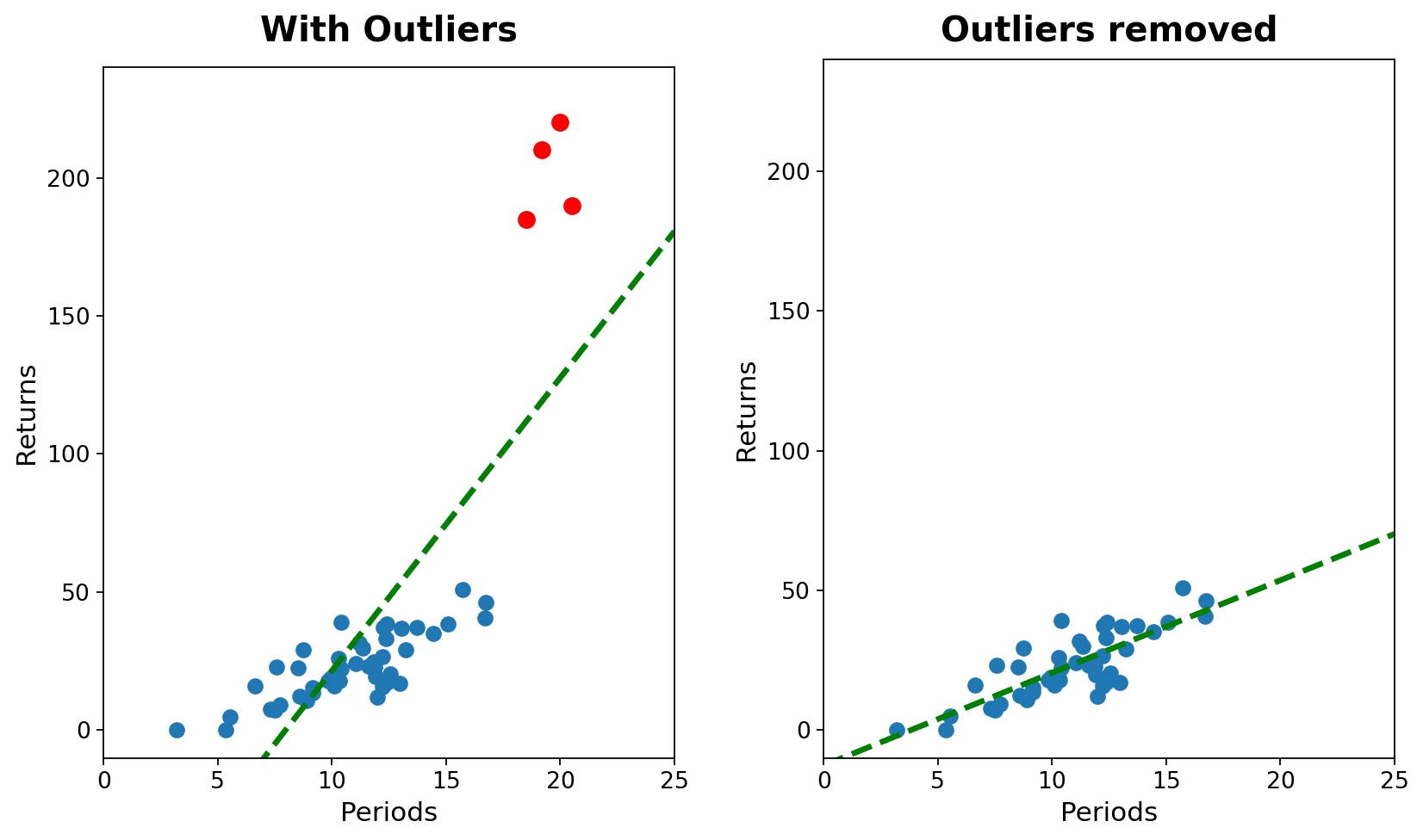
We require a method that is invariant to these eccentricities—a robust estimator with a high breakdown point that ignores the tails to focus on the structure.

Point 2: The RANSAC algorithm construction

We adopt the RANSAC (Random Sample Consensus) algorithm. RANSAC fundamentally transforms the regression problem from an optimization task (minimizing global error) into a search task (maximizing local consensus). It operates on the assumption that the data consists of inliers (points that can be explained by a model) and outliers (points that cannot).

Instead of trying to fit all points simultaneously, RANSAC iterates through a hypothesize-and-verify loop:

1. Hypothesize (minimal sampling): The algorithm randomly selects the smallest possible subset of data points required to analytically determine the model parameters. For a linear model in 2D space (time vs. PnL), this is exactly 2 points. These two points define a candidate line L_k.

2. Verify (consensus building): The algorithm tests this candidate line L_k against the entire dataset. It computes the residuals r_i for all data points i=1 … N. A point is classified as an inlier if its residual falls within a strict tolerance band δ (the residual_threshold):

   \(\mathbb{I}_{inlier}(i) = \begin{cases} 1 & \text{if } |y_i - \hat{y}_i| < \delta \\ 0 & \text{text{otherwise}} \end{cases}\)

   Crucially, in our implementation, δ is not arbitrary. It is derived robustly using the Median Absolute Deviation of the residuals, ensuring the threshold scales dynamically with the strategy’s baseline volatility.

3. Score and update: The score of the model is simply the cardinality of the consensus set (the count of inliers).

   \(\text{Score}(L_k) = \sum_{i=1}^N \mathbb{I}_{inlier}(i)\)

   We store the model with the highest score found so far.

4. Optimize (refinement): After iterating for K trials, we take the best consensus set found (e.g., 90% of the data) and re-run a standard regression only on those inliers. This polishes the fit, removing the jitter introduced by the minimal sampling in step 1.

The number of iterations K (max_trials) is determined probabilistically. If w is the probability that any given data point is an inlier, and we want a probability p (e.g., 99%) that at least one of our random samples consists entirely of inliers (yielding a “clean” model), we need:

\(K \geq \frac{\log(1-p)}{\log(1-w^n)}\)

where n=2 for a line. Even with substantial contamination (e.g., 20% outliers), RANSAC converges rapidly to the true structure of the PnL, identifying the steady accumulation of alpha while ignoring the shock events that confuse OLS.

Let’s implement this class: