[WITH CODE] Options: Straddles and strangles

Strategies with options Part III

---

Table of contents:

1. Introduction.

2. Limitation and risks.

3. Option strategies vs “regular” strategies.

4. Technical decomposition of strategies.

   1. Payoff geometry.

   2. Expected PnL as a function of realized volatility.

   3. Delta-hedged straddles.

   4. Skew and asymmetric exposure in strangles.

   5. Strike optimization for strangles (interior optima).

   6. Regime selection and entry policy.

   7. Correlation and capacity.

---

Before you begin, remember that you have an index with the newsletter content organized by clicking on “Read full story” in this image.

---

Introduction

Let's get straight to it. Anyone with a basic options textbook knows what a straddle or a strangle looks like. You buy a call and a put, and you hope for a big move. Simple, right? Well, no. The gap between that textbook diagram and a consistently profitable, scalable long-volatility strategy is immense. It's a chasm filled with mathematical nuance, microstructure friction, and behavioral traps. The questino here is pretty simple: How do we actually profit from these strategies? Although we can do additional questions like: Are they really profitable? When and how much?

The first and most critical realization for any practitioner is that straddles (long at-the-money (ATM) call + long ATM put, same expiry) and strangles (long out-of-the-money (OTM) call + long OTM put, same expiry) are not straightforward bets on price direction. They are, at their core, trades on the relationship between two different kinds of variance: the market's expectation of future variance, and the variance that actually materializes.

This immediately splits the problem into two primary modes of operation, each with its own PnL drivers and risks:

1. The buy and hold approach: In this mode, you buy the structure and hold it until expiration. Your PnL is elegantly simple to define:

   \(\text{PnL} = \text{Payoff}(S_T) - \text{Premium}_{\text{paid}}\)

   The premium you pay is a direct function of the options' implied volatility (IV), along with other factors like interest rates, dividends, and the specific shape of the volatility surface (i.e., skew and smile). To turn a profit, the underlying price at expiry, S_T, must have moved far enough away from the strike(s) to overcome the initial cost. Your profit is therefore contingent on the realized price dispersion being greater than the implied price dispersion you paid for. The dilemma here is that you are paying a premium that already embeds the market's consensus forecast for a large move. You are, in effect, betting that the consensus is wrong and that the future will be even more volatile than priced in.

2. The delta-hedged or variance engine approach: This is the far more common approach on institutional desks. Instead of holding a static position, you actively manage it by delta-hedging. By continuously buying or selling the underlying asset to keep the portfolio's delta near zero, you transform the nature of the trade. The PnL is no longer primarily about the final price S_T, but about the path taken to get there. The PnL decomposes into a stream of gains and losses:

   \(\text{PnL} \approx \sum (\text{Gamma Gains}) - \sum (\text{Theta Decay}) - \sum (\text{Hedging Costs}) \)

   You are monetizing the convexity (gamma) of your position by trading the underlying's movements, collecting small profits each time you re-hedge. Your enemy is time decay (theta) and the friction of transaction costs. Here, you are making a bet on the realized variance of the path versus the implied variance, modified by the costs of your hedging activity.

Review this presentation if you want more information:

Straddles And Strangles

1.58MB ∙ PDF file

Download

Download

Both of these modes are legitimate paths to potential profitability. Both can also be systematic ways to lose money if implemented with naïve assumptions. The core dilemma is not choosing between betting on direction vs. betting on volatility; it's a far more subtle conflict between variance monetization and variance taxation. The market taxes you through the premium (which reflects implied volatility), the constant bleed of theta, the microstructure frictions of hedging (bid-ask spreads, market impact), and the asymmetric costs embedded in the volatility skew. You monetize variance through the realized price path and the convexity of your option position. The entirety of this paper is about quantifying and optimizing this trade-off.

Limitation and risks

What, specifically, can go wrong? Before we build anything, we need a risk register. A quant who doesn't start with risk is just a gambler with a compiler. Here is the minimum viable risk map for any long straddle or strangle strategy:

1. Most liquid underlyings, particularly equity indices, exhibit a persistent Implied Volatility Risk Premium (IVRP)—implied–realized gap risk. This means that, on average, implied volatility is higher than the subsequent realized volatility. This premium exists because options are used for hedging and market participants are willing to pay a premium for downside protection. If you indiscriminately buy straddles or strangles, you are systematically paying this premium. You are on the wrong side of a structural market flow. Your strategy must have a mechanism for identifying regimes where this gap is likely to close or invert.

2. When you delta-hedge, your PnL depends critically on the path of the underlying, not just the start and end points—hedging path risk aka path dependency. A volatile, choppy market where you frequently re-hedge can generate substantial gamma gains. A slow, trending market with few reversals can lead to losses, as theta decay outstrips the infrequent gamma capture. The worst-case scenario is a large, overnight price gap (a jump), which your delta hedge completely misses, leaving you with a large unhedged loss.

3. A vanilla Black-Scholes model assumes constant volatility across all strikes. This is patently false. Market volatility surfaces are curved ("smile") and asymmetric ("skew"). For equity indices, downside puts are almost always more expensive in IV terms than equidistant upside calls. This means a strangle is not a symmetric bet. You are paying more for the downside wing, which raises your breakeven point and makes the trade's PnL asymmetric. A shift in the skew can dramatically alter your position's mark-to-market value, even if the underlying price and overall volatility level remain unchanged.

4. The most obvious time to buy a straddle is before a known event like a corporate earnings announcement or a central bank policy decision—event contingency risk. The problem is, this is obvious to everyone. The implied volatility for options expiring just after the event will be massively inflated. The market is pricing in the fireworks. Often, the actual price move—the realized fireworks—is smaller than what was implied. Buying a straddle can be like buying a lottery ticket after the price has been raised to reflect the jackpot size. The expected value can easily be negative.

5. Theory is clean; execution is messy. The further out-of-the-money you go for a strangle, the wider the bid-ask spreads and the thinner the liquidity. The price you see on the screen may not be the price you can trade at in any significant size. Furthermore, when you need to hedge most—during a volatile move—the liquidity in the underlying asset itself can dry up, causing your hedging costs (slippage and market impact) to skyrocket.

6. In calm market regimes where realized volatility is low, a long volatility position is a negative carry trade. You are paying out theta every single day. This steady bleed can lead to a significant drawdown over time. When your options approach expiry, you must decide whether to roll the position to a later expiration. This involves closing the old position and opening a new one, incurring transaction costs and potentially locking in a new premium at unfavorable levels.

7. All of our analysis relies on models. If we use a simple Geometric Brownian Motion model with constant volatility to design and test our strategies, our results will be misleading. Real asset prices exhibit regime-switching volatility, jumps, and stochastic volatility (volatility of volatility). Using an oversimplified model can cause you to systematically underestimate risks or overestimate potential profits.

We will confront each of these risks head-on with mathematics and simulation in the sections that follow.

Option strategies vs “regular” strategies

What makes volatility strategies fundamentally different from regular investment strategies? A regular equity portfolio is typically built around a core of long beta (market exposure), perhaps with factor tilts (like value, momentum, or quality). Its performance is dominated by directional price movements and its primary risk budget is allocated to market risk.

Straddles and strangles, especially when delta-hedged, operate in a different universe. Their risk budget is allocated to variance risk. Their performance driver is not whether the market goes up or down next month, but the magnitude and character of its fluctuations along the way.

This creates the pivotal conflict: You cannot evaluate or manage volatility strategies using the same models, metrics, or intuitions that apply to directional strategies.

1. A successful month for a long-stock portfolio is when the price ends higher. A successful month for a hedged straddle is when the path was volatile, regardless of where the price ended.

2. The Sharpe ratio of a directional strategy depends on its mean return versus its standard deviation. The information ratio of a volatility strategy depends on its ability to generate alpha from the variance risk premium.

3. Risk management for a directional portfolio focuses on controlling beta and drawdowns from market downturns. Risk management for a volatility portfolio focuses on controlling theta decay, vega exposure, and hedging friction.

Accepting this fundamental difference is the prerequisite for success. It forces a complete shift in research workflow, diagnostic tooling, and risk policy. It's the event that separates the dabblers from the systematic quants. All of this presents a new scenario with a series of questions that must be answered.

1. When to enter? What specific, quantifiable market conditions suggest that future realized variance is likely to exceed the currently implied variance, net of all expected costs? This is the regime selection problem.

2. What structure to use? Should we use a straddle or a strangle? If a strangle, how wide should the wings be? This is the strike selection and optimization problem.

3. Which expiry to choose? Should we use short-dated options to maximize gamma or longer-dated options to reduce theta decay and roll costs? This is the tenor selection problem.

4. How to manage the position? Should we hold to expiry or delta-hedge? If we hedge, what is the optimal hedging frequency or threshold to balance gamma capture against transaction costs? This is the dynamic management problem.

5. How to size the position? How much capital should be allocated to any given trade, based on its expected edge, its risk profile, and its correlation with the rest of our portfolio? This is the risk allocation problem.

6. How to control leakage? How do we design our execution logic to minimize slippage, market impact, and spread costs, which can easily erode a small theoretical edge? This is the microstructure problem.

With this roadmap established, we now proceed to the seven technical points that form the heart of our quantitative treatment.

Technical decomposition of strategies

Before we can run, we must walk. The foundational step is to precisely define the instruments and their sensitivities. While this may seem basic, a surprising number of errors stem from a fuzzy understanding of these fundamentals.

A. Payoff geometry

Let's be precise. A European option's value depends on the spot price S, strike price K, risk-free interest rate r, continuous dividend yield q, time to expiration T, and implied volatility sigma.

1. Long straddle (ATM):

   This strategy involves buying one call option and one put option with the same expiration date (T) and the same strike price (K), where (K) is chosen to be at-the-money (ATM), i.e., (K ≈ S₀), the spot price at initiation.

   The payoff at expiration, given a final stock price (S_T), is the sum of the payoffs of the call and the put:

   \(\text{Payoff}_{\text{straddle}}(S_T) = (S_T - K)^{+} + (K - S_T)^{+} = |S_T - K|\)

   The net PnL is this payoff minus the initial premium paid (Pi₀):

   \(\text{PnL}_{\text{straddle}}(S_T) = |S_T - K| - \Pi_0\)

   This creates the characteristic V-shape payoff diagram.

2. Long strangle (OTM):

   This strategy involves buying one call option and one put option with the same expiration date (T), but with different strike prices. The call strike, (K_c), is chosen to be out-of-the-money (OTM), so (K_c > S₀). The put strike, (K_p), is also chosen to be OTM, so (K_p < S₀).

   The payoff at expiration is:

   \(\text{Payoff}_{\text{strangle}}(S_T) = (S_T - K_c)^{+} + (K_p - S_T)^{+}\)

   The net PnL is this payoff minus the initial premium paid (Π₀):

   \(\text{PnL}_{\text{strangle}}(S_T) = (S_T - K_c)^{+} + (K_p - S_T)^{+} - \Pi_0\)

   This creates a U-shaped or bucket-shaped payoff diagram, as the region between (K_p ) and (K_c ) results in a total loss of the premium.

The premium Π₀​ is usually calculated using an option pricing model, most commonly the Black–Scholes–Merton framework. For a European call option, the model considers factors such as:

\(C(S, K, r, q, \sigma, T) = S_0 e^{-qT} \Phi(d_1) - K e^{-rT} \Phi(d_2)\)

• The current underlying price S₀

• The strike price K

• Time to maturity T

• The risk-free interest rate r

• Any dividend yield q

• The volatility σ of the underlying asset

In the BSM model, the call price is obtained by combining the present value of the expected gain from exercising the option with the probability of it finishing in the money. These probabilities come from the standard normal distribution, and are determined by two parameters (d₁ and d₂​) that account for time, volatility, and the relationship between the current price and the strike price.

\(d_1 = \frac{\ln(S_0 / K) + \left(r - q + \frac{1}{2}\sigma^2\right)T}{\sigma \sqrt{T}}, \quad d_2 = d_1 - \sigma \sqrt{T}\)

The price of a put option can be computed with the same approach, or more simply, by using the put–call parity relationship, which links the prices of calls and puts with the same strike and expiry.

\(P = C - S_0 e^{-qT} + K e^{-rT}\)

We won't go into defining the Greeks because that's something you can find in previous articles in more detail.

[WITH CODE] Options: Iron Condor

[WITH CODE] Options: Iron Butterfly

Breakeven levels at expiry

The breakeven points are where the terminal payoff equals the initial premium paid.

1. For a straddle with strike K and premium Π₀, the two breakeven points at expiry are:

   \(S_{BE, \text{up}} = K + \Pi_0 \quad \text{and} \quad S_{BE, \text{down}} = K - \Pi_0 \)

2. For a strangle with strikes K_p, K_c and premium Π₀, the breakevens are:

   \(S_{BE, \text{up}} = K_c + \Pi_0 \quad \text{and} \quad S_{BE, \text{down}} = K_p - \Pi_0 \)

   The strangle has a wider range of unprofitable outcomes between its breakeven points, but this is compensated for by a lower initial premium Pi_0.

The following snippet generates the payoff diagram:

import numpy as np
from scipy.stats import norm

# Black-Scholes Pricer (European) 
def bs_price(S, K, r, q, sigma, T, option_type="call"):
    """Calculates Black-Scholes price for a European option."""
    if T <= 0 or sigma <= 0:
        return np.maximum(0.0, S - K) if option_type == "call" else np.maximum(0.0, K - S)
    
    d1 = (np.log(S / K) + (r - q + 0.5 * sigma**2) * T) / (sigma * np.sqrt(T))
    d2 = d1 - sigma * np.sqrt(T)
    
    if option_type == "call":
        price = S * np.exp(-q * T) * norm.cdf(d1) - K * np.exp(-r * T) * norm.cdf(d2)
    else: # put
        price = K * np.exp(-r * T) * norm.cdf(-d2) - S * np.exp(-q * T) * norm.cdf(-d1)
    return price

# Parameters 
S0 = 100.0  # Initial stock price
r = 0.05    # Risk-free rate
q = 0.02    # Dividend yield
T = 30 / 365 # Time to expiration (30 days)
iv = 0.25   # Implied volatility

# Straddle Calculation 
K_straddle = 100.0
call_premium_straddle = bs_price(S0, K_straddle, r, q, iv, T, "call")
put_premium_straddle = bs_price(S0, K_straddle, r, q, iv, T, "put")
premium_straddle = call_premium_straddle + put_premium_straddle

# Strangle Calculation 
K_put_strangle = 95.0
K_call_strangle = 105.0
call_premium_strangle = bs_price(S0, K_call_strangle, r, q, iv, T, "call")
put_premium_strangle = bs_price(S0, K_put_strangle, r, q, iv, T, "put")
premium_strangle = call_premium_strangle + put_premium_strangle

# Payoff Calculation 
S_T = np.linspace(70, 130, 200) # Range of prices at expiry
payoff_straddle = np.maximum(S_T - K_straddle, 0) + np.maximum(K_straddle - S_T, 0)
pnl_straddle = payoff_straddle - premium_straddle

payoff_strangle = np.maximum(S_T - K_call_strangle, 0) + np.maximum(K_put_strangle - S_T, 0)
pnl_strangle = payoff_strangle - premium_strangle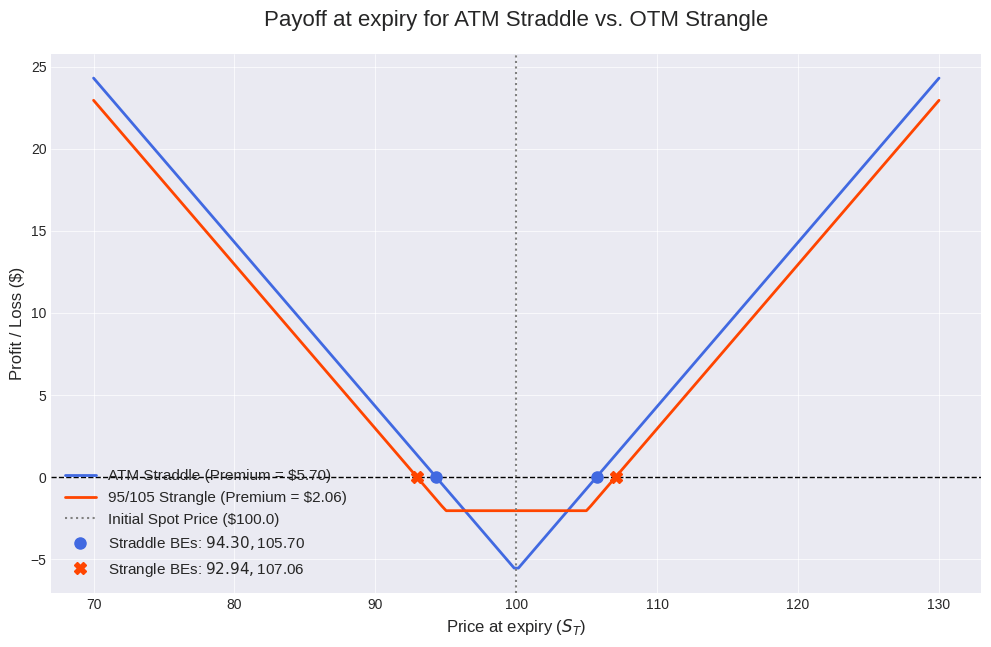

The plot clearly shows the straddle's tighter breakeven points and higher premium versus the strangle's wider, cheaper structure.

Pitfall #1: "A straddle is just a bigger, more aggressive version of a strangle."

This is a dangerous oversimplification. They are fundamentally different instruments from a risk management perspective. A straddle's PnL is most sensitive to realized volatility very close to the current price. A strangle's PnL is driven by larger deviations and is far more sensitive to the shape of the volatility surface (skew), as the two wings are priced at different points on the smile. The cost structure, gamma profile over the price path, and sensitivity to skew are distinct. They require different optimization and hedging logic. Treat them as separate tools for different jobs.

B. Expected PnL as a function of realized volatility

The static payoff diagram is useful, but it doesn't tell us anything about the probability of ending up at any given point. To make an informed decision, we need to analyze the strategy's expected PnL under different assumptions about the future. The most important assumption is the volatility that the underlying will actually realize over the life of the options.

Let’s frame the problem: we buy a straddle or strangle priced with a certain implied volatility, σ_i. We then hold it to expiration. The world unfolds, and the underlying asset exhibits a realized volatility of σ_r. The question is: what is our expected PnL as a function of σ_r?

Analytically solving for the expected payoff E[|S_t − K|] under the physical measure with lognormal returns is possible but cumbersome. A far more practical and flexible approach is Monte Carlo simulation, where we simulate thousands of possible price paths for the underlying asset using a given realized volatility σ_r and calculate the average PnL.

We model the stock price using Geometric Brownian Motion, the same model underlying Black-Scholes. A price path is simulated as:

\(S_{t+\mathrm{d}t} = S_t \exp\left( \left( \mu - \frac{1}{2} \sigma_R^2 \right) \mathrm{d}t + \sigma_R \sqrt{\mathrm{d}t} \, Z \right) \)

Where μ is the expected return (under the physical measure, we’ll use r−q for simplicity),
σ_r is the realized volatility we are testing, and Z is a standard normal random variable.

The process is:

1. Fix the strategy (e.g., a 30-day ATM straddle) and calculate its premium, Π₀, using a fixed implied volatility (e.g., σ_i = 25).

2. Choose a grid of possible realized volatilities to test (e.g., σ_r in [5]).

3. For each σ_r in the grid:
   a. Simulate a large number (N) of price paths to expiration T.
   b. For each path, calculate the terminal payoff of the strategy.
   c. Compute the average payoff across all N paths.
   d. The expected PnL is this average payoff minus the fixed premium Π₀.

4. Plot the expected PnL against the realized volatility σ_r.

Let’s implement this simulation.

# Monte Carlo Simulation Engine 
def simulate_paths(S0, mu, sigma, T, steps, n_paths):
    """Simulates GBM price paths."""
    dt = T / steps
    Z = np.random.normal(size=(n_paths, steps))
    increments = (mu - 0.5 * sigma**2) * dt + sigma * np.sqrt(dt) * Z
    log_paths = np.cumsum(increments, axis=1)
    # Start paths at S0
    S = np.hstack([np.full((n_paths, 1), S0), S0 * np.exp(log_paths)])
    return S

# Simulation Parameters 
n_paths = 50000
steps = 30
vol_grid = np.linspace(0.05, 0.80, 31) # Realized vol from 5% to 80%

# Premiums are fixed based on IV=25%
iv_pricing = 0.25
prem_straddle = bs_price(S0, K_straddle, r, q, iv_pricing, T, "call") + \
                bs_price(S0, K_straddle, r, q, iv_pricing, T, "put")
prem_strangle = bs_price(S0, K_call_strangle, r, q, iv_pricing, T, "call") + \
                bs_price(S0, K_put_strangle, r, q, iv_pricing, T, "put")

# Run the Simulation 
expected_pnl_straddle = []
expected_pnl_strangle = []

for realized_vol in vol_grid:
    # Simulate final prices
    S_paths = simulate_paths(S0, r - q, realized_vol, T, steps, n_paths)
    S_T = S_paths[:, -1]
    
    # Calculate expected payoffs
    exp_payoff_straddle = np.mean(np.maximum(S_T - K_straddle, 0) + np.maximum(K_straddle - S_T, 0))
    exp_payoff_strangle = np.mean(np.maximum(S_T - K_call_strangle, 0) + np.maximum(K_put_strangle - S_T, 0))
    
    # Calculate expected PnL
    expected_pnl_straddle.append(exp_payoff_straddle - prem_straddle)
    expected_pnl_strangle.append(exp_payoff_strangle - prem_strangle)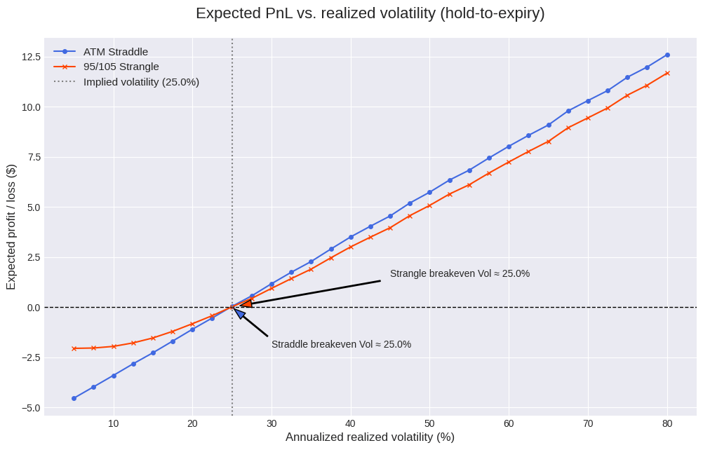

The plot is revealing the basis for any systematic long-volatility strategy.

1. Monotonic relationship: The expected PnL for both strategies is a monotonically increasing function of realized volatility. This is the entire premise of the trade.

2. The breakeven volatility: For each strategy, there is a critical value of realized volatility at which the expected PnL crosses from negative to positive. This is the volatility hurdle. In our simulation, where options were priced with an IV of 25%, the straddle needs realized volatility to be slightly above 25% to break even on average. This is because of the concavity of the option payoff with respect to volatility (Jensen's inequality). The relationship is not exactly E[PnL]>0 if and only if σ_R>σ, but for at-the-money options, it’s a very close approximation.

3. Straddle vs. Strangle: The strangle's curve sits below and to the right of the straddle's. It costs less, but it requires a significantly higher realized volatility to become profitable. However, at very high levels of realized volatility, the slope of the strangle's PnL curve can become steeper, indicating higher leverage to extreme moves.

The key takeaway is that a hold-to-expiry strategy is essentially a bet on the difference between the square of realized volatility and the square of implied volatility. If your forecast for realized volatility is higher than the market’s implied volatility, the trade has a positive expectancy before accounting for forecast error. However, if you have no view and the implied volatility is consistently higher than the average realized volatility (because of the implied volatility risk premium), the trade will systematically lose money.

Pitfall #2: "Event weeks are guaranteed money-makers for straddles."

Events are only profitable if the actual outcome's volatility exceeds the implied volatility, which is already massively inflated ahead of the event. For many scheduled events (like earnings for mega-cap stocks), the market is remarkably efficient at pricing the expected move. The IV often over-prices the median move, meaning you lose money on the typical outcome. To profit, you need the event to be a true surprise that generates a move in the tail of the distribution, or you need a systematic way to identify when the IV is mispriced even by event standards. Simply buying straddles into every event is a recipe for paying the IVRP to the sellers.

C. Delta-hedged straddles

Now we move to the more interesting approach: treating the straddle as a variance engine. Why would we do this? Holding to expiry exposes us to a single binary outcome at T. By delta-hedging, we can monetize the volatility of the path itself, effectively collecting a stream of small gains throughout the option's life.

When we maintain a delta-neutral portfolio, our PnL is no longer driven by the final stock price, but by the interplay of gamma, theta, and costs. The discrete-time PnL from re-hedging at intervals of Δ_T

\(\text{PnL} \approx \sum_{t=1}^N \left( \frac{1}{2} \Gamma_t (\Delta S_t)^2 - \Theta_t \Delta t \right) - \sum_{t=1}^N \text{Cost}_t \)

1. Gamma gains: The term ½ Γ_t (ΔS_t)² represents the profit from the option’s convexity. Being long gamma means we make money on price changes in either direction. This term is directly proportional to the squared return — the realized variance — and reflects how we harvest volatility.

2. Theta decay: The term −Θₜ Δt is the cost of holding the position over one time step. This is the deterministic loss (bleed) that must be overcome.

3. Costs: The term Costs_t represents transaction costs (such as spreads and slippage) incurred each time we re-hedge. More frequent hedging captures gamma more accurately but also increases total costs.

The goal of a delta-hedged strategy is to find periods where the expected gamma gains will exceed the sum of theta decay and hedging costs. Talk is cheap. Let's simulate it. We'll take a 1-month ATM straddle and simulate its PnL when delta-hedged daily. We'll run two experiments: one with zero transaction costs (an idealized market) and one with a realistic proportional cost of 5 basis points (0.05%) on the value of every hedge trade.

# Delta Hedging Simulation Engine 
def bs_delta(S, K, r, q, sigma, T, option_type="call"):
    """Calculates Black-Scholes delta."""
    if T <= 0:
        return 1.0 if S > K else 0.0 if option_type == "call" else -1.0 if S < K else 0.0
    d1 = (np.log(S / K) + (r - q + 0.5 * sigma**2) * T) / (sigma * np.sqrt(T))
    return np.exp(-q * T) * norm.cdf(d1) if option_type == "call" else -np.exp(-q * T) * norm.cdf(-d1)

def delta_hedged_pnl_straddle(S0, K, r, q, T, iv, steps, n_paths, txn_cost_perc=0.0, seed=42):
    """Simulates PnL for a delta-hedged straddle."""
    np.random.seed(seed)
    dt = T / steps
    # We simulate under the implied vol for this example
    S_paths = simulate_paths(S0, r - q, iv, T, steps, n_paths)
    
    # Initial cost of the straddle
    premium = bs_price(S0, K, r, q, iv, T, "call") + bs_price(S0, K, r, q, iv, T, "put")
    
    pnl = np.zeros(n_paths)
    for i in range(n_paths):
        S = S_paths[i, :]
        cash_account = 0.0
        stock_position = 0.0
        
        # Initial hedge
        delta_target = bs_delta(S[0], K, r, q, iv, T, "call") + bs_delta(S[0], K, r, q, iv, T, "put")
        stock_position = delta_target
        cash_account -= stock_position * S[0]
        cash_account -= abs(stock_position) * S[0] * txn_cost_perc

        # Daily re-hedging
        for t in range(1, steps):
            tau = T - t * dt
            delta_target = bs_delta(S[t], K, r, q, iv, tau, "call") + bs_delta(S[t], K, r, q, iv, tau, "put")
            
            trade_amount = delta_target - stock_position
            cash_account -= trade_amount * S[t]
            cash_account -= abs(trade_amount) * S[t] * txn_cost_perc
            stock_position = delta_target
            
        # Final settlement
        final_option_value = np.maximum(S[-1] - K, 0) + np.maximum(K - S[-1], 0)
        final_stock_value = stock_position * S[-1]
        
        pnl[i] = (final_option_value + cash_account + final_stock_value) - premium
        
    return pnl

# Run Simulations 
pnl_no_cost = delta_hedged_pnl_straddle(S0, K_straddle, r, q, T, iv, steps, 10000, txn_cost_perc=0.0)
pnl_with_cost = delta_hedged_pnl_straddle(S0, K_straddle, r, q, T, iv, steps, 10000, txn_cost_perc=0.0005) # 5 bps cost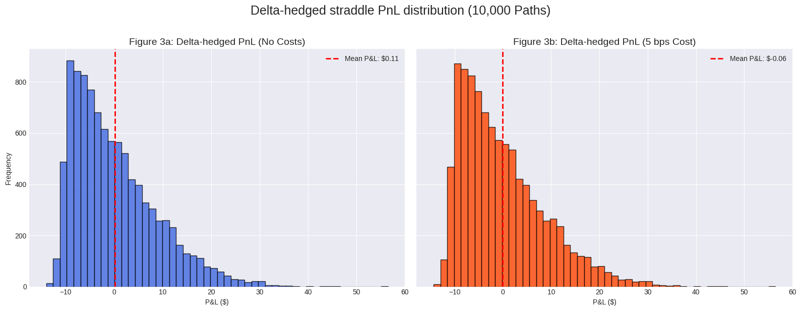

The histograms tell a clear story.

• Without costs: The PnL distribution is centered very close to zero. This is what we expect when the realized volatility of our simulation (25%) matches the implied volatility used for pricing (25%). The trade is, on average, a fair game. The distribution has fat tails, representing paths with very high or very low realized variance.

• With costs: The entire distribution shifts to the left. The mean PnL is now significantly negative. This leftward shift represents the total transaction costs paid over the life of the strategy. This is the variance taxation in its most direct form. The 5 bps cost, which seems small on any single trade, creates a systematic drag on performance that turns a fair game into a losing one.

This simulation proves that for a delta-hedged strategy, cost control is not an optimization, it's a prerequisite to avoid bankruptcy. Your process must either (a) select only those periods where expected gamma gains are high enough to overcome this cost drag, or (b) implement a more intelligent hedging scheme. For example, instead of hedging on a fixed time interval (daily), one could use a threshold-based approach: only re-hedge when the portfolio's delta deviates by more than a certain amount (epsilon). This reduces turnover in quiet periods while remaining responsive during volatile moves. Calibrating this epsilon is a key part of strategy design.

Pitfall #3: "Delta-hedged straddles are safe because they are market-neutral."

"Market-neutral" does not mean risk-free. It's one of the most misused phrases in finance. A delta-hedged straddle has simply exchanged its first-order directional risk for a complex set of other risks. You are now explicitly short theta (you lose money every day), long gamma (you are exposed to the variance of returns), long vega (exposed to shifts in IV), and critically, you are exposed to jump risk (a large gap that your hedge cannot capture) and transaction cost risk. The risk hasn't vanished; it has just changed form.

D. Skew and asymmetric exposure in strangles