


Table of contents:
Introduction.
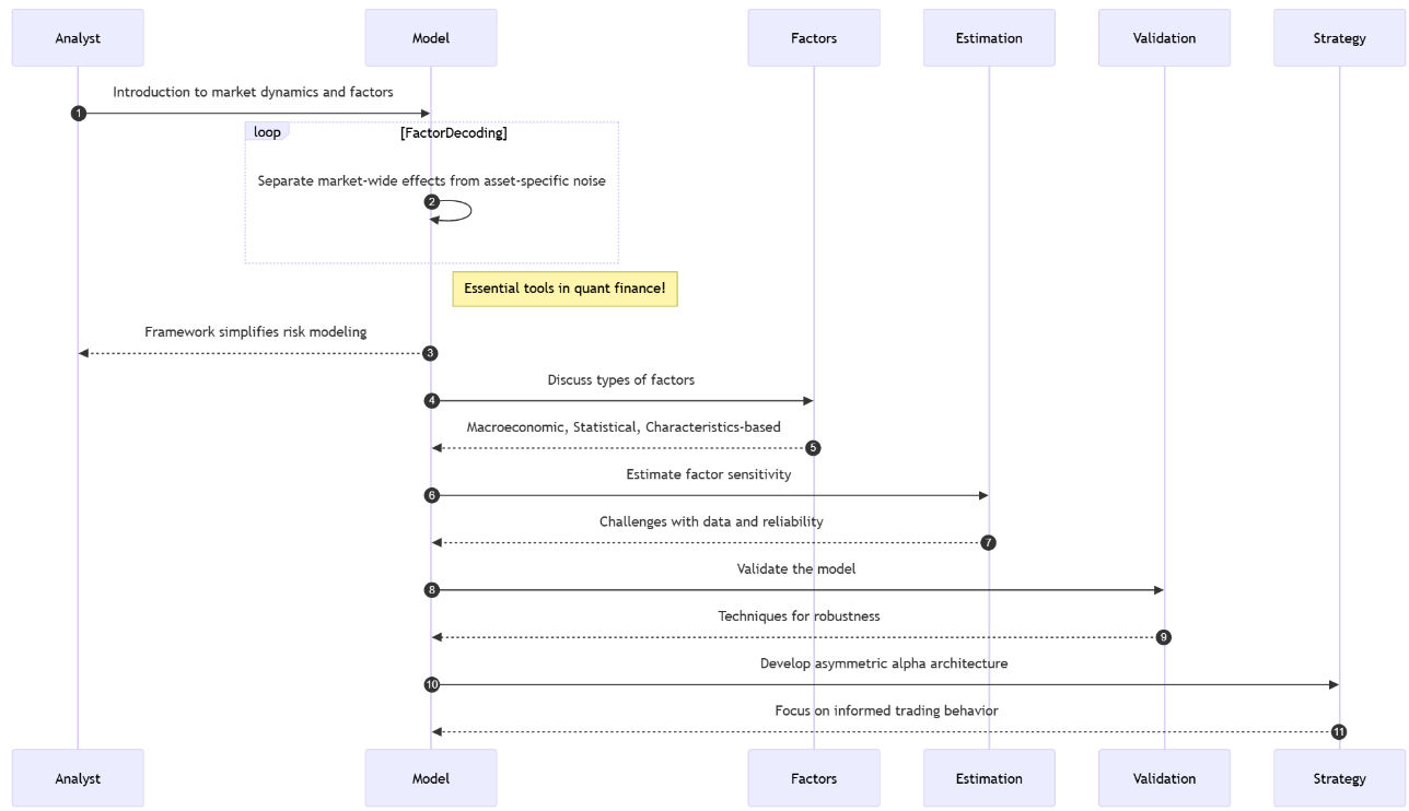
Modeling framework development.
Factor selection.
Parameter estimation.
Model validation.
Asymmetric alpha architecture.
Before you begin, remember that you have an index with the newsletter content organized by clicking on “Read the newsletter index” in this image.

Introduction
Let me tell you about this fascinating puzzle in quantitative finance. You see individual stocks bouncing around like hyperactive electrons, right? But squint at the market long enough, and you start noticing this strange synchronicity–like they’re all humming along to some hidden melody. Which makes you wonder: how the hell do we model this group dance mathematically?
Now, modeling each asset in isolation? That’s financial fantasyland. It’s like assuming every instrument in an orchestra plays without sheet music. Reality? They’re all responding to the same conductors – interest rates, inflation shocks, that useless Trump tweet that tanked SP500 again. This is why we factor model nerds exist.
Let me break it down. Factor models are basically financial x-ray vision. I’m saying any asset’s return is really two things mashed together: stuff everyone’s exposed to—we call these factors—plus security-specific noise. Think of it like this—Do you remember this equation? We saw it in a previous post:
Translation: Your return rₜ is some baseline alpha, plus your factor exposures B times factor moves fₜ, plus whatever weirdness is unique to that stock εₜ. Simple equation, right? But here’s where it gets sexy–the covariance structure:
This bad boy reveals market risk’s DNA. The first term? That’s your systematic risk – the market forces we all swim in. The second term? That’s the idiosyncratic stuff you might actually diversify away. Beautiful, but…
[Pauses dramatically] …here’s where PhD students start crying. Four landmines await:
Specification risk: Choose factors that miss latent drivers? It’s like building a weather model that ignores atmospheric pressure. Your tech stock factor might completely whiff on AI revolution dynamics, leaving you blind to concentrated exposures.
Estimation risk: That delicious-looking 20% factor loading? Might be statistical mirage. Financial data’s signal-to-noise ratio makes particle physics look clean–sampling errors compound, turning elegant math into overfit fiction.
Non-stationarity risk: Markets have the memory of a goldfish. Today’s ironclad factor relationship—value vs. growth, anyone?—might invert tomorrow when macro regimes shift. Your backtested beauty becomes a real-time liability.
Multicollinearity risk: When factors bleed together – say, "quality" and "low volatility" doing an interpretive dance–your beta coefficients become Schrödinger’s parameters: simultaneously significant and meaningless.
Yet despite all this? We still use these models. Because when they work–when you nail the factors, tame the noise, respect the instability – you’re not just predicting returns. You’re seeing the market’s hidden skeleton.
Modeling framework development
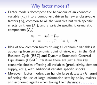
Let’s start by observing market synchronicity to constructing a robust factor model is one of translating empirical patterns into a rigorous mathematical framework. The core conceptual leap, captured by the expression rₜ = α + Bfₜ + εₜ, is the decision to model the multivariate return vector not as n independent variables, but as a system driven by a smaller set of m common forces fₜ, mediated by a sensitivity matrix B, with residual asset-specific movements ϵₜ. This is the narrative about the idea–the quest to find the hidden levers that move the market.
Check more about this here:
In this framework:
rₜ is the vector of excess returns for n assets at time t.
α is the vector of asset-specific intercepts—often interpreted as alpha, though its estimation is fraught.
fₜ is the vector of factor returns at time t, where m≪n.
B is the factor loading matrix, quantifying the sensitivity of each asset to each factor. Bij represents the loading of asset i on factor j.
ϵₜ is the vector of idiosyncratic returns at time t.
The power of this linear decomposition lies in its ability to separate systematic risk—driven by fₜ and B—from idiosyncratic risk—captured by ϵₜ. This separation is not merely academic; it is fundamental to risk management and portfolio construction in algorithmic trading.
The elegance of the framework is amplified by a crucial assumption where the idiosyncratic returns are uncorrelated with the factor returns, and are also uncorrelated with each other across assets.
Mathematically:
where Ωϵ is a diagonal matrix.
This assumption, while simplifying the mathematics, represents a significant obstacle in practice. Markets often exhibit subtle, time-varying correlations even in residual terms, challenging the diagonal nature of Ωϵ.
Under these assumptions, the covariance matrix of asset returns, Ωr, takes on its canonical decomposed form we saw in the introduction and where
is the covariance matrix of the factors.
This equation is the engine of the factor model. It states that the total covariance between assets is the sum of the covariance driven by their shared factor exposures and the covariance arising from their independent idiosyncratic movements.
This decomposition offers a potent solution to the curse of dimensionality that plagues covariance estimation in large portfolios. A full n×n covariance matrix requires estimating n(n+1)/2 unique parameters. For n=1000 assets, this is nearly half a million parameters!
A factor model with m=10 factors, however, requires estimating nm elements for B, m(m+1)/2 elements for Ωf, and n elements for the diagonal Ωϵ. This significantly reduces the number of parameters, making estimation more tractable and less prone to error, especially with limited historical data.
The reduction is dramatic.
However, building this engine involves multiple obstacles:
The first is factor selection: what are the right factors? Are they macroeconomic variables, statistical constructs, or characteristics of the assets themselves? Each choice introduces its own set of assumptions and challenges.
The second is parameter estimation: accurately estimating B, Ωf, and Ωϵ from noisy, non-stationary financial data is a non-trivial task.
The third is validation: how do we rigorously test if our factor model is truly capturing the market's systematic structure or merely fitting historical noise?
These obstacles transform the elegant mathematical framework into a complex engineering challenge, demanding careful consideration at every step.

Factor selection
Choosing the right factors is a scientific discovery guided by economics, statistics, and sometimes, intuition. Do we use macroeconomic variables like interest rate changes or inflation surprises? Do we extract statistical factors using techniques like Principal Component Analysis? Or do we rely on asset characteristics like value, momentum, or size, inspired by empirical observations like the Fama-French factors?
Each choice carries its own baggage:
Macroeconomic factors: Directly linked to economic variables—e.g., changes in inflation, interest rates, GDP growth. They are intuitive but often suffer from low frequency, revision risk, and potential lag between the event and market reaction. Example: A surprise increase in interest rates impacting bond proxies and financials.
Statistical factors: Derived purely from the covariance structure of returns using techniques like Principal Component Analysis. PCA identifies orthogonal linear combinations of assets that explain the maximum variance. While statistically optimal for capturing covariance, the resulting factors may lack economic intuition and their interpretation can shift.
Characteristic factors: Based on observable asset characteristics—e.g., Price-to-Book ratio for Value, market capitalization for Size, past returns for Momentum, debt-to-equity for Quality. These are inspired by empirical anomalies or theoretical risk premia but are susceptible to data mining and the risk that the premium disappears once discovered and arbitraged away.
Choosing factors that miss key drivers is like navigating by stars on a cloudy night. If the rise of AI is a major market force, and your factor model lacks an adequate tech innovation factor—perhaps implicitly captured, but poorly—you might severely underestimate the correlated risk within a portfolio of AI-exposed stocks. This is the heart of specification risk–building a model that fundamentally misrepresents the underlying market structure.
For these reasons I like to use vola factors. Let’s code a method to identify them:
import numpy as np
import pandas as pd
from sklearn.linear_model import LinearRegression

# 1) SIMULATE SYNTHETIC DATA
np.random.seed(42)

t = 500   # time periods
n = 10    # number of assets
m = 3     # number of factors

# factor returns (t × m)
factor_returns = np.random.normal(scale=1.0, size=(t, m))

# true loadings B (n × m)
true_B = np.random.uniform(low=0.5, high=1.5, size=(n, m))

# idiosyncratic noise (t × n)
epsilon = np.random.normal(scale=0.5, size=(t, n))

# asset returns: R = F·Bᵀ + ε  → shape (t × n)
R = factor_returns @ true_B.T + epsilon

# for clarity, optional DataFrames
dates   = pd.date_range(start="2020-01-01", periods=t, freq="D")
assets  = [f"Asset_{i+1}" for i in range(n)]
factors = [f"Factor_{j+1}" for j in range(m)]

df_R = pd.DataFrame(R, index=dates, columns=assets)
df_F = pd.DataFrame(factor_returns, index=dates, columns=factors)

# 2) ESTIMATE LOADINGS VIA CROSS‐SECTIONAL REGRESSION
estimated_B = np.zeros((n, m))
for i in range(n):
    model = LinearRegression().fit(df_F.values, df_R.iloc[:, i].values)
    estimated_B[i, :] = model.coef_

# 3) COMPUTE SYSTEMATIC RETURNS (t × n)
sys_R = factor_returns @ estimated_B.T

# 4) COMPUTE VARIANCES PER ASSET (axis=0)
var_total       = R.var(axis=0)       # shape (n,)
var_systematic = sys_R.var(axis=0)   # shape (n,)

# 5) FRACTION OF VARIANCE EXPLAINED
explained_ratio = var_systematic / var_total
# sanity check: all values should be between 0 and 1, no NaNs
print("Explained variance ratios:", np.round(explained_ratio, 3))

output = {"assets": assets, "explained_ratio": np.round(explained_ratio, 3).tolist()}
The output would be:
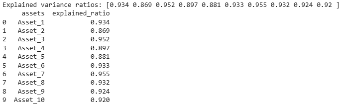
Here we see how variability could explain which factor to choose. But it's not the only method; ideally, one should choose one that matches the nature of the factor—the data must be consistent with the method.
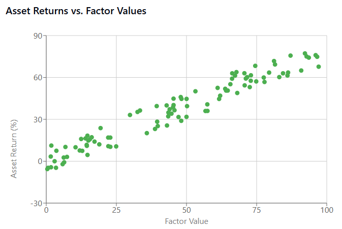
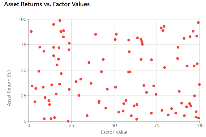
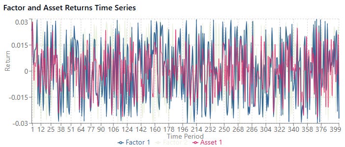
For example if we visualize a strong factor, it shows a clear linear relationship between the factor and asset returns. This suggests the factor captures a genuine market dynamic that could be exploited.
A poor factor exhibits a random cloud pattern, indicating no meaningful relationship. Using this factor would introduce specification risk as it doesn't capture any relevant market dynamics.
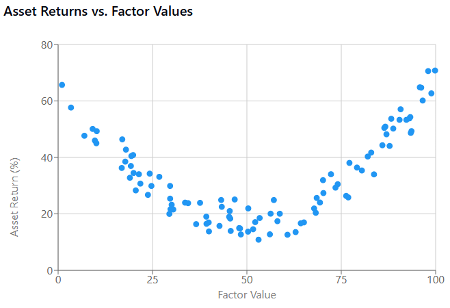
Besides, some factors have nonlinear relationships with returns. Traditional linear models might miss these patterns, creating another type of specification risk.
Parameter estimation
Even with factors chosen, accurately estimating the factor loadings matrix B and the factor covariance matrix Ωf from noisy, finite financial data is a formidable task. The standard approach often involves running time-series regressions for each asset against the chosen factors to estimate the loadings.
Consider a simple multiple linear regression for a single asset i:
Estimating the β coefficients via Ordinary Least Squares seems straightforward:
where R is the matrix of asset returns and F is the matrix of factor returns. However, financial data has a notoriously low signal-to-noise ratio. Outliers, structural breaks, and simple random fluctuations can heavily influence these estimates. The delicious-looking 20% factor loading might indeed be a statistical mirage, an artifact of estimation error rather than a true, stable exposure.
Furthermore, estimating Ωf requires estimating the covariance matrix of the factors themselves. While m≪n, factors can still be correlated, and estimating their covariance matrix from limited data introduces further estimation risk.
Let’s simulate some noisy data following a factor model structure and then estimate the parameters using OLS. Show how estimation error can occur with limited data.
import numpy as np
import pandas as pd
import statsmodels.api as sm
# Simulate data
np.random.seed(42)
T = 100 # Time periods (limited data)
m = 2 # Number of factors
n = 10 # Number of assets
# Simulate factor returns (e.g., market and size factors)
F = np.random.randn(T, m)
F = sm.add_constant(F, prepend=True) # Add constant for alpha
# Simulate true factor loadings and alpha
true_alpha = np.random.randn(n, 1) * 0.001 # Small alpha
true_B = np.random.randn(n, m) * 0.1 # True loadings
true_params = np.hstack((true_alpha, true_B))
# Simulate idiosyncratic noise
epsilon = np.random.randn(T, n) * 0.005 # Small idiosyncratic risk
# Simulate asset returns
R = F @ true_params.T + epsilon
# Estimation
# Estimate parameters for each asset
estimated_params = []
for i in range(n):
model = sm.OLS(R[:, i], F)
results = model.fit()
estimated_params.append(results.params)
estimated_params = np.array(estimated_params)
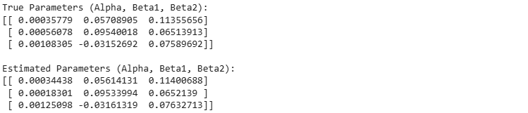
print("True Parameters (Alpha, Beta1, Beta2):")
print(true_params[:3, :]) # Print for first 3 assets
print("\nEstimated Parameters (Alpha, Beta1, Beta2):")
print(estimated_params[:3, :]) # Print for first 3 assets
# Note: With T=100, the estimates will likely be quite different from true values
# This snippet illustrates the concept of estimating B via regression for each assetThe output would be:
Something to keep in mind:
How factor loadings are estimated from financial data.
The impact of sample size on estimation accuracy.
How noise levels affect parameter estimation.
For example, a small sample, low noise levels and beta size achieved these results:
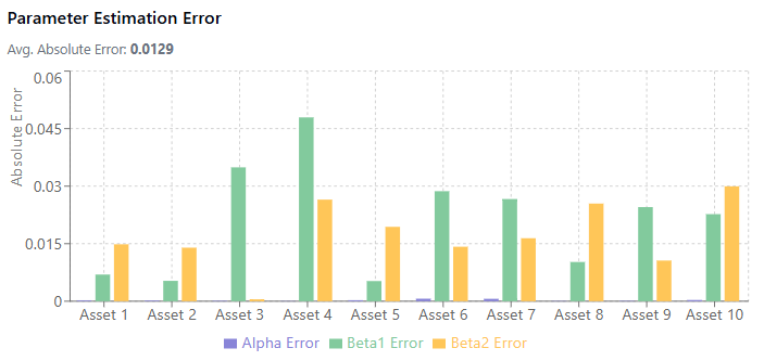
Versus a bigger sample, higher noise and beta size:
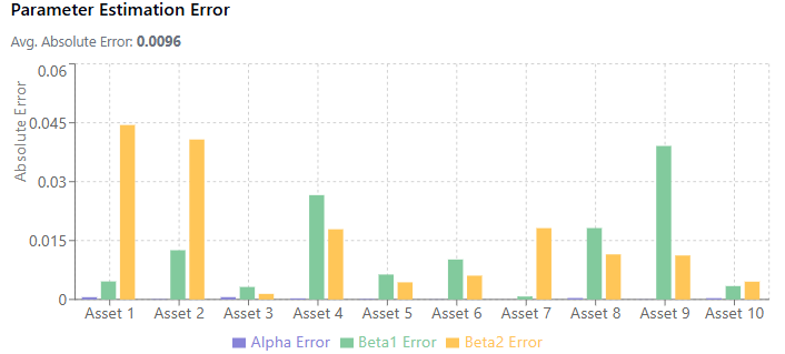
Damn! So ugly!
When the noise level is high relative to the beta size, estimates become much less reliable. This is the low signal-to-noise ratio problem in financial data.
While not directly visualized, the estimation of the factor covariance matrix Ωf introduces additional estimation risk, especially when factors are correlated.
Model validation
Validating a factor model's performance is a perpetual challenge. Standard backtesting involves testing the model on historical data not used in estimation. But given the non-stationarity of markets, a model that fit historical data well might fail to predict future relationships. How do you rigorously test if your model is capturing enduring systematic structure versus simply overfitting to past noise?
The fundamental paradox lies in trying to validate a model designed to predict dynamics in a non-stationary future using only the static record of a past that may not repeat itself. A model can fit historical data exquisitely, capturing all its nuances and patterns, yet fail catastrophically when faced with a new market regime, an unprecedented shock, or a fundamental shift in relationships. This isn't just a challenge, it's an existential threat to the model's utility, where performance relies on accurate, forward-looking inputs.
Standard backtesting, which involves estimating the model on one historical period—the in-sample data—and evaluating its performance on a subsequent, distinct period—the out-of-sample data—is a necessary first step but is profoundly insufficient on its own. It can tell you if the model had explanatory power over a specific past period it didn't see during training, but it provides limited assurance that those relationships will hold in the future.
Robust validation requires a multi-faceted approach, examining different aspects of the model's performance and assumptions:
How much of the variation in asset returns—either over time for a single asset or across assets at a single point in time—does the model actually explain? This is often measured by R2. High time-series R2 for an individual asset regression indicates its returns are strongly driven by the factors. High cross-sectional R2 at a given time indicates that the factor exposures effectively explain the differences in returns across assets at that moment.
While high R2 is desirable–it suggests the factors are capturing common variance–it is a measure of fit, not necessarily predictive power. A model can have high historical R2 by overfitting to noise or temporary relationships.

Are the estimated factor loadings Bij statistically significant? Standard t-tests on the regression coefficients are used here.
A statistically insignificant loading suggests that, based on the historical data, you cannot confidently say the asset has exposure to that factor. Beyond statistical significance, the loadings should also be economically sensible.
Does the sign and magnitude of a stock's beta to the energy factor align with what you know about the company? Inconsistent or illogical loadings can signal model misspecification, data errors, or multicollinearity.
How well does the model predicts future returns ak alpha and, crucially, future risk aka covariance? Predicting alpha is notoriously difficult due to its low signal-to-noise ratio. Validating risk predictions is more tractable and often the primary goal of factor models in practice.
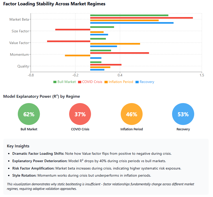
The inherent difficulty is that a model validated on data from the 2018s might fail to capture the dynamics of a 2020s market shaped by new technologies, pandemics, and geopolitical shifts. The market's memory is short, and its structure is fluid.
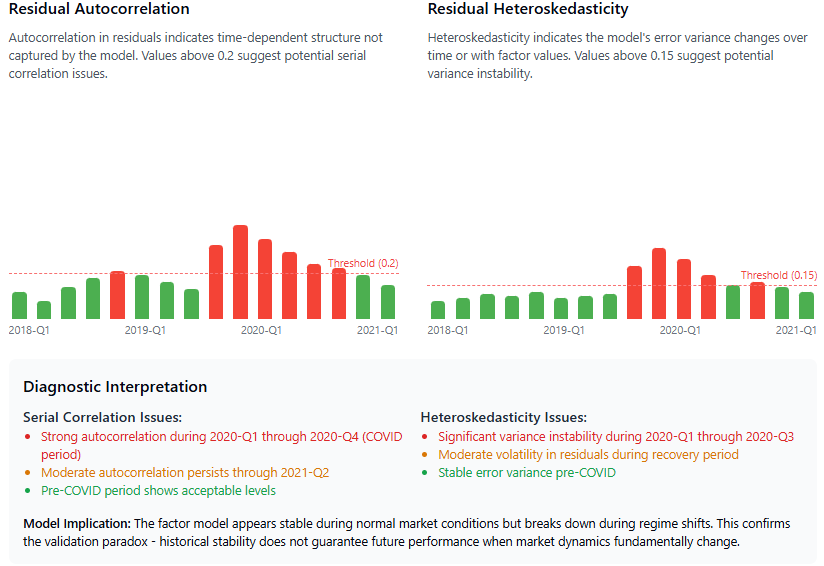
The resolution to this paradox lies in adopting dynamic validation methodologies that acknowledge and simulate this non-stationarity. Some of the minimum and sanity tests would be:
Explanatory power.
Significance test.
Residual analysis and diagnostics.
Rolling window validation.
Walk-forward validation.
Regime-based validation.
Monte Carlo robustness.
Of course, there are more, and you don't have to use all of the above. Choose a combination that checks a minimum of the factor properties.