

[WITH CODE] Risk Engine: Position manager
Is it a good idea to make partial closes? How should you go about closing positions that remain open when risk increases?

Table of contents:
Introduction.
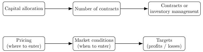
Risk identification from the framework.
Data drift as foundation.
Drift-based position management.
Implementation and development.
Performance determinants and behavioral modalities.
Before you begin, remember that you have an index with the newsletter content organized by clicking on “Read full story” in this image.

Introduction
In the day-to-day grind of systematic trading, volatility isn’t just a market feature—it’s the atmosphere we operate in. It drives the edge, defines the risk, and sets the tempo. But while volatility creates the conditions for profit, it also contains the seeds of our destruction. That tension—between opportunity and ruin—sits at the heart of every execution cycle. And that’s precisely why I set out to build a lightweight yet responsive framework for managing inventory in mid-to-low frequency trading systems. Nothing fancy—just something simple, adaptive, and tuned to volatility.
Indeed, this is the third part of a Risk Engine I have created.
You can check previous parts here:

Let’s ground it. Say a model throws a clean signal, confidence is high, and we go in with meaningful size. Price moves in our favor—briefly. Then macro erupts, implied vols shoot up, and the PnL curve starts to resemble a polygraph hooked to a liar. We’re still “right” on the thesis, but the path is now disorderly. What does the system do? Hold and hope the thesis plays out? Or unwind and minimize risk? This isn’t a thought experiment—it’s the moment where edge dies or survives.
This isn't a code problem—it’s a framework problem. Static stop-losses? Too crude. They cut not because you’re wrong, but because volatility breathes too loudly. Full-hold strategies? Too naive. They're what blowups are made of. Most position managers operate in binaries: you're in or you're out. But volatility isn’t binary—it’s a spectrum. It requires probabilistic response, not deterministic rules.
That’s where volatility-aware inventory control kicks in. But it’s not free. The minute you try to adapt to volatility, you inherit Parameterization Risk. The thresholds that define when to size up, trim, or bail out become your weak spot. Too tight, and the system flinches at every noise burst—paying the spread, burning commissions, and self-sabotaging its own exposure. Too loose, and it watches in horror as drawdowns swell. Precision matters, but overfitting kills. It’s a calibration puzzle with no permanent solution.
Then comes the reactivity-stability Tradeoff. The framework needs to detect real regime shifts—vol going from baseline to panic mode—while filtering transient flickers. That’s not easy. React too fast and you’re fragile. React too slow and you’re useless. Every smoothing filter introduces lag. Every lag reduces reactivity. You’re trapped in a delay/robustness paradox. The trick is tuning just enough to catch structural volatility changes, while staying deaf to noise.
Now throw in the discrete nature of most tradable instruments. A system may recommend reducing exposure by 0.67 contracts—great in theory. But markets deal in integers. You can’t slice a futures contract. That creates granularity-induced friction. If your sizing logic depends on continuous outputs, but your broker demands integer volume, you'll get mismatches. Small inefficiencies compound. In worst cases, no trade happens when it should.
Another hidden bomb: the framework is only as good as the signals it manages. It's not a strategy—it’s an optimizer. If your signal is built on noise, the manager becomes a beautiful machine executing garbage. No matter how clever the risk logic, it cannot salvage a bad entry model. This kind of framework is a convex amplifier: it scales what’s already there. Garbage in, leveraged garbage out.
But the real trigger for the framework’s necessity is when volatility becomes unstable. Not just high vol—volatile vol. You see it around central bank events, geopolitical shocks, systemic dislocations. The variance of variance spikes. It’s no longer about whether volatility is elevated—it’s about the structure of that volatility. Is it trending up? Oscillating? Breaking pattern? That meta-volatility layer breaks simple rules. You can't rely on fixed thresholds. You need adaptability that tracks not just the state of volatility, but its derivative, convexity, and duration.
That’s where this framework earns its keep. By adjusting dynamically to both the level and the behavior of volatility, it becomes more than a position manager—it becomes a volatility interpreter. That was the crux that pushed me to build this system: a lightweight, volatility-sensitive adjustment mechanism that responds not only to price action, but to the volatility of volatility itself. The moment vol became unpredictable was the moment a static rulebook stopped working. This was my answer.

Risk identification from the framework
But even with this adaptive backbone in place, the framework isn’t bulletproof. There are structural limitations in the actual implementation that still need to be addressed:
The model treats drift as a simple first-order delta in VIX (
v - prev_v). This is effective in capturing local pressure changes but completely blind to volatility curvature. If the volatility is increasing steadily across a window, the model sees only a series of small drifts, never recognizing the acceleration. This causes late reactions to compounding risk. A better formulation would estimate the second derivative—convexity of volatility—or integrate over a rolling drift window to detect compounding exposure build-up.Current closure logic is time-agnostic: it sees only the present drift and current size. But the age of a position matters. A position held through six hours of turbulence is very different from one just opened. Without tracking time-in-position or cumulative exposure, the system lacks temporal pressure awareness. Introducing inventory aging logic or exposure-duration decay would allow the framework to recognize when positions have overstayed their welcome.
Due to granularity constraints, fractional close recommendations often get rounded down and ignored. But the system forgets those micro-intentions. Over time, this leads to slippage between modeled vs. actual exposure. A residual buffer mechanism—accumulating unexecuted close fractions—would let the system act once those add up to a tradable size, tightening tracking precision.
The framework reacts smoothly to volatility changes, but binary signal shifts (1→0) result in immediate, full position closures, regardless of drift, VIX, or ongoing dynamics. This abruptness contradicts the otherwise probabilistic design. A better solution would involve soft signal fading, using transition probabilities or a de-escalation ramp rather than instantaneous exits, especially under neutral volatility conditions.
All trades are treated equally in conviction—signal equals 1, full entry; signal equals 0, full exit. But signals themselves often vary in confidence: overlapping triggers, statistical strength, or model ensemble agreement. The system lacks a mechanism to scale position sizing by signal certainty, leading to overexposure on weak edges and underutilization on strong ones. Adding a confidence-weighted contract scaler would enhance risk efficiency.
As you can see, there's a lot of room for improvement in this prototype. We'll see how to fix it in future versions. For now, I suggest you try to find a way to improve it!

Data drift as foundation
Data drift arises when the statistical properties of the input variables used in a model evolve over time. Conceptually, it’s akin to navigating with a map that no longer matches the terrain: your coordinates may be technically correct, but the landmarks have shifted. In the context of trading systems, especially those sensitive to macro and volatility signals like the VIX, data drift is not just a nuisance—it’s a structural risk to inference accuracy and decision-making.
Let X be the input feature vector. During model development, we assume that the training data is drawn from a probability distribution P1(X), and that this distribution remains stable at inference time. However, in practice, the distribution often changes, and this is the essence of data drift:
This discrepancy implies that any learned function f(X), which performed well under P1(X), may degrade significantly under P2(X), especially when the model is overly reliant on patterns or correlations specific to the training regime.
In financial terms, this is particularly important when your model relies on inputs like the VIX, which encapsulate implied volatility and are highly reactive to market sentiment, geopolitical shifts, and systemic shocks.
Here more about the different types of drift:

While several taxonomies exist, in the context of a VIX-driven model, we restrict our attention to the two most relevant drift mechanisms:
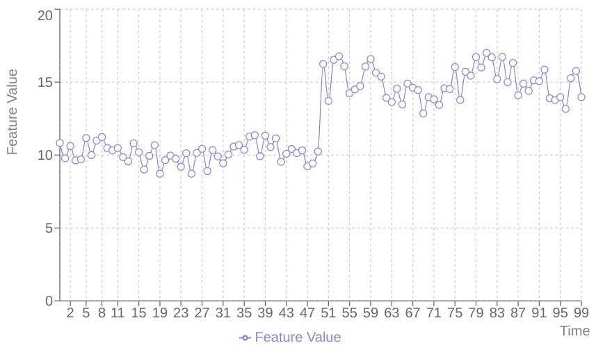
Sudden drift or abrupt regime shift:
This type of drift represents an instantaneous change in the underlying data-generating process. It often reflects structural breaks due to macro events—central bank interventions, liquidity crises, or regime changes in volatility dynamics.
Formally, this can be expressed as:
\(f(x)_{t+1} = \begin{cases} f(x)_t, & \text{if } t < t_0 \\ g(x)_t, & \text{if } t \ge t_0 \end{cases}\)Where:
f(x)t: the pre-drift data-generating function.
g(x)t: the post-drift function.
t0: the moment of distributional shift.
A volatility model trained on a low-VIX regime fails catastrophically when volatility spikes due to a geopolitical shock. The model still believes it's operating in a calm market, but reality has shifted to a turbulence regime.Gradual drift or slow tansition:
In this case, the change in the distribution occurs progressively. This can happen when market conditions evolve due to shifting risk sentiment, changes in investor positioning, or the slow decay of previous volatility regimes.
A convex combination of past and emerging distributions models this well:
\(f(x)_t = (1 - \alpha(t)) \cdot f(x)_0 + \alpha(t) \cdot g(x)\)Where:
α(t)∈[0,1] is a monotonically increasing function such that α(t)→1 as t→∞.
f(x)0: the original data-generating process
g(x): the target distribution the data is drifting toward
As volatility slowly rises due to an ongoing inflation crisis, the statistical profile of the VIX changes. A model that adapts its sensitivity gradually can continue to perform reasonably well—if and only if the drift is detected in time.
Here an example, the ditribution changes while maintaining the same underlying relationship:
And here another example where the properties change while maintaining the underlying distribution:

Drift-based position management
The conceptual bedrock of adaptive drift-based position management is the transformation of market volatility from a static state variable into a dynamic process variable. Instead of merely observing the level of volatility, we track its momentum, its rate of change. This is the core idea: to measure the "drift" in volatility, much like a sailor gauges the drift of their vessel due to currents and winds.
Mathematically, this begins with a straightforward measurement. If vt represents the market's volatility index—like the VIX or an instrument-specific equivalent—at a given time t, the raw, instantaneous volatility drift at that moment is simply the difference from the previous observation:
This raw measure, however, is inherently noisy. It captures every tiny fluctuation, every market gasp and sigh. Acting directly on this raw drift would lead to the skittish, over-reactive behavior we seek to avoid. To smooth out this noise and discern the underlying trend in volatility, we employ an Exponential Moving Average. The EMA gives more weight to recent observations while still incorporating historical data, providing a smoothed trajectory of volatility change:
Here, α is the smoothing factor, typically calculated as α=2/(n+1), where n is the lookback window size. A larger n results in a smaller α, providing more smoothing but also introducing more lag. This formula is the digital equivalent of observing a cloud's slow, deliberate movement across the sky rather than focusing on the frantic fluttering of its edges.
The conventional position management paradigm often relies on static, pre-defined thresholds. If volatility crosses X, reduce position; if it crosses Y, exit. This is like setting a single tripwire and hoping the intruder steps exactly there. Our framework ascends beyond this static limitation through the implementation of dynamic thresholds. The threshold for initiating position adjustments is not a fixed number; it is a value that adapts to the prevailing market environment.
The dynamic threshold is calculated using a blend of factors:
In this equation:
base_thresholdprovides a foundational level of sensitivity, a default tripwire setting.s is the sensitivity parameter (0≤s≤1), controlling how much the current volatility level vt influences the threshold. A higher s makes the threshold more responsive to current market anxiety.
0.1⋅smoothed_driftt is a momentum component. If volatility is accelerating upwards—positive smoothed drift—the threshold increases slightly, demanding a stronger signal—larger raw drift—to trigger a position reduction. This prevents over-reaction to moderate but sustained volatility increases. Conversely, if smoothed drift is negative, the threshold decreases, making the system more sensitive to potential upward volatility spikes during a generally calming period.
This dynamic calculation creates an adaptive tripwire that is low in calm markets—allowing positions to ride with less risk of premature exit—but rises with market anxiety, requiring more significant volatility shocks to trigger action when the market is already agitated. It's a sophisticated lock that adjusts its tumblers based on the perceived threat level.
Furthermore, we're assuming our system only opens long positions. If it also opens short positions, we'll need to modify the function logic or multiply the VIX by -1.
Once the system determines that a position reduction is necessary based on the relationship between the raw drift and the dynamic threshold, the next step is determining how much of the position to close. A simple linear relationship—e.g., close 10% for every point of drift above the threshold—can be too abrupt or too slow depending on the scale.
The framework utilizes an Exponential-Saturation model for position sizing. This approach creates a non-linear response, where the fraction of the current position to close follows a curve:
Here, max_close_fraction is the maximum percentage of the initial position that can be closed in a single step—though in implementation, it's applied to the current position to prevent closing more than available. The term (1−e^−raw_drift/threshold) is the exponential saturation part. Let's break down its cleverness:
When draw_drift/threshold is small—drift is only slightly above the threshold—the exponent is close to zero, e0=1, so 1−e0=0. This means tiny drifts result in near-zero closing fractions–a crucial feature for ignoring minor fluctuations and respecting granularity.
As raw_drift/threshold increases, the exponential term e^−ratio decreases towards zero. The term (1−e^−ratio) grows, approaching 1.
This creates a curve where position reduction starts slowly, accelerates through medium-sized drifts, and then saturates. Even very large drifts—relative to the threshold—won't push the fraction beyond
max_close_fraction. This prevents closing the entire position too easily and maintains some exposure unless an extreme, abrupt condition is met.
This exponential curve is like a progressively tighter grip:
A gentle squeeze for small concerns, a firm hold for moderate issues, and maximum pressure applied only when the situation becomes genuinely alarming.
Finally, the calculated theoretical position reduction must confront the pragmatic reality of granularity integration. Financial instruments aren't infinitely divisible. You trade whole contracts, whole shares, or specific lot sizes. The framework handles this by rounding the desired reduction amount to the nearest valid trading increment:
Here, initial_contracts is the position size originally opened, and min_contract is the smallest tradable unit for the instrument. This calculation scales the desired fractional close amount by the initial position size to get a nominal number of contracts, rounds this number to the nearest multiple of the minimum contract size, and returns this adjusted amount.