Would you be able to pass a quant interview?
How far do you have to go to compete against a mediocre quant team? Let's look at a Citadel interview question
Table of contents:
Introduction.
How to face this type of problems?
Probability basics.
Random variables and expected value.
Fair games in probability.
Sequential games in probability.
Clarifying possible strategies.
First-principles approach to expected value.
What is the expected number of opens?
Solution for the fair cost.
Introduction
You're in an interview for Citadel, one of the largest funds in the world. Your hands are sweating, your mouth is dry, and you're moving like a headless chicken.
They're going to give you a short test to filter out undesirable candidates. You're scared, you're nervous, and yet you're telling yourself positive messages like "You can do it, you can do it, come on...!"
It's going to be a short 40-question test, and it will take just under an hour to answer them.
Here's the first one:
It's been 45 minutes... it wasn't as hard as it seemed, right!? Or was it!? 👽
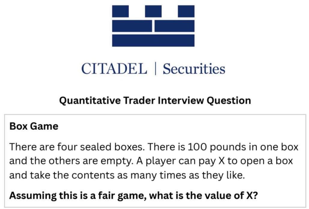
The box game puzzle asks:
Given four sealed boxes with exactly one box containing £100, and a fee X for each box you open, what is the value of X that makes this a fair game (i.e., the expected net gain is zero)?
Despite its surface simplicity, the puzzle touches upon core ideas in probability and decision theory, such as the relationship between information gained—learning which box is empty—and the reduction in uncertainty about the prize’s location. From a broader standpoint, this problem connects to:
Expected value: A fundamental concept in probability theory that helps quantify the average outcome of a random process over many trials.
Decision theory: Particularly, sequential decision making under uncertainty. Once a box is opened and found empty, the decision maker updates their knowledge about the location of the prize.
Fair games: In gambling or finance, a fair game is one in which the expected net outcome is zero. Any difference from zero implies a systematic advantage—positive EV—or disadvantage—negative EV.
In a single round, the chance of success is 1/4. If that fails, the next attempt has probability 1/3 of success, and so on, until eventually, if all else fails, the final box is guaranteed to have the money. Understanding how these probabilities aggregate—and how the cost accumulates—lies at the heart of the puzzle.
How to face this type of problems?
Before diving into it, it is worth ensuring we have a firm grasp of fundamental probability concepts. While many readers will be familiar with these, stating them explicitly helps unify our language and clarifies each building block of the argument.
Probability basics
In the context of this puzzle:
Sample space: The set of all possible outcomes of an experiment. Here, the sample space for Which box has the £100? has 4 equally likely possibilities.
Event: A subset of the sample space. For instance, the event Box #1 has the £100 is one possible outcome with probability 1/4.
Conditional probability: Once we open a box and see it is empty, the probabilities of the remaining boxes containing the £100 must be updated accordingly.
If you want to continue discovering more about this staff, don’t miss this section:
Random variables and expected value
A random variable is a function that assigns numerical values to outcomes. In the Box Game, we have two primary random variables:
W: The total winnings from the game. If you find the £100, W=100W = 100W=100; if, hypothetically, the money is never found—not really possible here if you keep opening boxes—it would be 0, but in practice you will always eventually find the £100 if you choose to continue.
C: The total cost you pay to open boxes. Each time you open a box, you pay X. If you open boxes nnn times, your total cost is n×X.
The expected value of a random variable Z is the average of Z over the probability distribution of all possible outcomes. Symbolically,
for discrete random variables, or an integral for continuous ones. In this puzzle, we deal with discrete random variables and finite sums.
Fair games in probability
A game is fair if the expected net outcome is zero. If G denotes the net gain/loss from the game—the total money you receive minus the total cost you pay—the fairness condition is:
When a puzzle asks, What cost X makes the game fair?, it is asking us to solve for X such that:
Sequential games in probability
This puzzle also exemplifies a sequential game, where the player makes decisions at each step—open a box or stop. After each step, the player gains information—whether that box was empty.
In an optimal play scenario, the player continues opening boxes until the £100 is found—since any rational player who has already paid for partial information is incentivized to keep going until they succeed.
Thus, from a purely logical standpoint, you would never stop early if you are playing for expected monetary value—assuming risk neutrality. The cost accumulates with each opened box, but so does the probability that the next open yields the prize.
Clarifying possible strategies
Let's start from the beginning and break down the key points.
There are 4 boxes in total. Exactly one of these boxes has £100, and the other 3 are empty.
The player does not know which box contains the money.
The player can pay X pounds to open a box.
Upon opening, if the box is empty, the player gains no money but learns that particular box definitely does not contain the £100.
The player may open as many boxes as desired. If they open a box and find the £100, they keep it.
The question is: what is the fair X? i.e., what X sets the game’s expected net gain to zero?
Because the boxes do not get “reset” or “shuffled,” once a box is found empty, it remains empty and does not revert to containing money. The memory of the player is perfect: you always know which boxes have been opened and the outcomes. This means with each empty box discovered, your knowledge of where the £100 is located becomes more precise.
Although the puzzle states that the player can open the same box multiple times, a rational strategy never involves re-opening a box known to be empty. Hence, the optimal approach is straightforward:
Open a box that has not yet been revealed.
If it has the £100, stop.
If it is empty, move on to another unopened box.
Continue until you find the money.
The cost for each box opening is X. If you find the money on the first try, you only pay X once. If you find it on the second try, you pay 2X, and so forth. If you are extremely unlucky, you might find the money in the last box, paying 4X.
First-principles approach to expected value
Let G be the net gain from playing this game exactly once, under the optimal strategy described above—which is effectively the only rational approach. Then:
The amount won is always £100—since we will eventually find the correct box if we keep playing. The total cost depends on how many boxes we open before finding the money. Let N be the random variable denoting the number of opens until we discover the prize. Then:
Hence,
Thus, the entire problem of computing E[G] boils down to finding E[N], the expected number of boxes we open.
Once we know E[N], the expected cost is X×E[N]. The expected payout is 100, since we always—eventually—get the £100. Therefore,
We can also think in a more direct way:
Probability you succeed on the first box: 1/4. Then net gain: 100−X.
If that fails—probability 3/4—you open a second box.
Probability that the second box is correct: 1/3 given the first was empty. Then net gain: 100−2X.
Probability that the second box is also empty: 2/3. Then you move on.
Third box: Probability 1/2 of success, net gain 100−3X. Probability 1/2 it is also empty.
Fourth box: Guaranteed success if you’ve opened three empties, net gain 100−4X.
So given these probabilities, the expected net gain E[G] can be written as:
Factor out 1/4:
Combine like terms:
We see that:
This directly shows that the puzzle’s outcome depends linearly on X. If X is too large, the game has negative expected value for the player; if X is small, the player gains an advantage.
For more of all of this:
What is the expected number of opens?
An equivalent perspective is: the expected number of box openings E[N] is 2.5. If you multiply that by X and subtract from 100, you get the net EV. Why 2.5?
You can think of it this way: each box has a 1/4 chance of being the correct one. On average, you “check” 2.5 boxes until you stumble on the correct one. Indeed, for a uniform random arrangement of 4 items, the average position of the winning item is:
This is a simpler argument: if you randomly place the prize among 4 distinct positions, the expected position is the mean of 1, 2, 3, and 4.
Another approach uses the concept of states:
Start in state S4—4 unknown boxes. The probability of success in each attempt is 1/4.
If you fail, you move to state S3—3 unknown boxes. Probability of success is 1/3.
If you fail, move to S2—2 unknown boxes. Probability of success is 1/2.
If you fail, you are in S1—1 box left. Probability of success is 1.
One can set up equations for the expected time to success in each state, leading to the same 2.5 result. This is a standard Markov chain or absorbing Markov process approach [Resource].
Solution for the fair cost
A fair game means the expected net gain is zero:
From our formula, E[G]=100−2.5X.
Hence: 100−2.5X=0.
Solve for X:
Thus, the cost per open that yields an expected net outcome of zero for the player is £40. If the game charges less than £40, the expected value to the player is positive; if it charges more, the expected value is negative.
Let’s see how to simulate that:
import numpy as np
import matplotlib.pyplot as plt
np.random.seed(2025)
def simulate_box_game(X, trials=1000000):
"""
Simulate the box game for a given cost X per open.
The function returns the average net gain over a number of trials.
"""
net_gain = np.zeros(trials)
for i in range(trials):
# There are 4 boxes; one of them has the prize.
boxes = [0, 0, 0, 0] # initialize all boxes as empty
prize_index = np.random.randint(0, 4)
boxes[prize_index] = 100 # assign prize
# Shuffle the boxes to simulate a random order
np.random.shuffle(boxes)
# Open boxes sequentially until the prize is found.
# 'opened' counts the number of boxes opened.
opened = 0
for value in boxes:
opened += 1
if value == 100:
break
net_gain[i] = 100 - opened * X
return np.mean(net_gain)
# Testing the simulation for a specific value of X
X_test = 40
avg_gain = simulate_box_game(X_test)
print("For X =", X_test, "the simulated average net gain is:", avg_gain)
Time to test this snippet. It runs the game for a given X over many trials and returns the average net gain. For X=40, you should see an average net gain very near zero, confirming the theoretical result—indeed 0.01444.
Next, we can plot how the expected net gain changes as a function of X. Recall that our theoretical expression is:
We can both plot this theoretical line and overlay simulation results.
# Define a range of X values to test
X_values = np.linspace(0, 80, 100)
simulated_gains = [simulate_box_game(X, trials=100000) for X in X_values]
# Compute theoretical expected net gain
theoretical_gains = 100 - 2.5 * X_values
# Create a plot comparing simulation to theory
plt.figure(figsize=(10, 6))
plt.plot(X_values, theoretical_gains, label='Theoretical EV (100 - 2.5X)', linewidth=2)
plt.scatter(X_values, simulated_gains, color='red', s=15, alpha=0.7, label='Simulated EV')
plt.axhline(0, color='black', linestyle='--')
plt.xlabel('Cost per open (X)', fontsize=12)
plt.ylabel('Expected net gain (EV)', fontsize=12)
plt.title('Expected net gain vs. cost per open (X)', fontsize=14)
plt.legend(fontsize=12)
plt.grid(True)
plt.show()
The output would be:
Here we can see the theoretical curve and the simulated data points. You should see that the simulation aligns closely with the straight line 100−2.5X.
While our main analysis focused on 4 boxes and a £100 prize, the concepts can be generalized. For nnn boxes:
The probability that the prize is in position k is 1/n.
The expected number of opens is:
\(\mathbb{E}[N] = \frac{1 + 2 + \dots + n}{n} = \frac{n+1}{2}\)The net gain would then be:
\(G = 100 - X \times \frac{n+1}{2}.\)Setting E[G]=0 gives:
\(X=\frac{200}{n+1}.\)
So what we have here can be implemented as:
def simulate_box_game_general(X, n=4, trials=100000):
"""
Simulate the box game for a general number of boxes 'n' and a given cost X.
One box out of n contains the prize (100). Returns the average net gain.
"""
net_gain = np.zeros(trials)
for i in range(trials):
boxes = [0] * n
prize_index = np.random.randint(0, n)
boxes[prize_index] = 100
# Shuffle the boxes to randomize the order of opening
np.random.shuffle(boxes)
opened = 0
for value in boxes:
opened += 1
if value == 100:
break
net_gain[i] = 100 - opened * X
return np.mean(net_gain)
# Choose different numbers of boxes and calculate the fair cost X = 200/(n+1)
n_values = [3, 4, 5, 6, 7]
fair_costs = [200/(n+1) for n in n_values]
# Simulate for each value of n and plot the fair cost predictions
simulated_fair_cost = []
for n in n_values:
# We search for X such that the average net gain is near zero.
# Here we assume the theoretical fair cost is accurate.
X_theoretical = 200/(n+1)
simulated_gain = simulate_box_game_general(X_theoretical, n=n)
simulated_fair_cost.append(simulated_gain)
print("For n =", n, "boxes, theoretical fair X =", X_theoretical, "simulated average net gain =", simulated_gain)
plt.figure(figsize=(10, 6))
plt.plot(n_values, fair_costs, marker='o', linestyle='-', color='blue', label='Theoretical fair cost')
plt.xlabel('Number of boxes (n)', fontsize=12)
plt.ylabel('Fair cost per open (X)', fontsize=12)
plt.title('Theoretical fair cost vs. number of boxes', fontsize=14)
plt.legend(fontsize=12)
plt.grid(True)
plt.show()
And after several iterations we would have:
The plot shows that as the number of boxes increases, the fair cost per open decreases.
Pretty cool eh!? There are more approaches to solve that like Bayesian view or Monte Carlo simulation. But the one that we checked it’s fine. Alright folks, that’s a wrap for today! Until next time—trade with logic and trust your data! 📊
PS: How valuable do you find mentorship or peer feedback for improving your algos?