[WITH CODE] Scale-free portfolio selection

A practical guide to implementing AdaHedge with L1 turnover caps and trust bands

---

Table of contents:

1. Introduction.

2. Risks and model limitations.

3. Online Portfolio Selection without knobs.

4. Mathematical framework.

   1. AdaHedge and AdaNormalHedge.

   2. The L1 turnover cap and trust band.

5. Why this breaks common misconceptions.

6. Algorithm design.

7. Strongly-adaptive aggregation and diagnostics.

---

Introduction

For decades, the world of quantitative portfolio management has been sitting on a fragile foundation. This isn’t a problem of bad math or weak computing power. It’s a problem of philosophy. Whether you’re running a small, nimble fund or a massive institutional book, the core problem is the same: your model is riddled with knobs.

These knobs are the parameters, the magic numbers that you, or some sophisticated optimization routine, painstakingly tuned to make your strategy look perfect on a historical backtest. They are the ghosts in the machine.

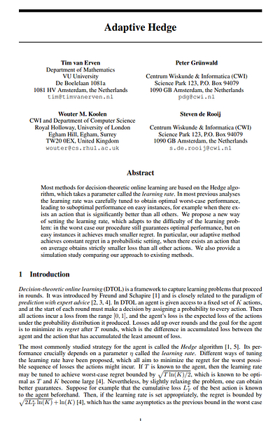
Let’s be specific, as this isn’t an abstract complaint. These are real, structural points of failure present in 99% of models. Perhaps the most critical is the learning rate, or η. In any gradient-based allocator, like Exponentiated Gradient or Online Newton Step, this knob dictates how fast your model learns from new information. If you tune η to be high, you get a fast, twitchy model that reacts instantly and gets whipsawed by every piece of market noise, churning your portfolio to dust. If you tune η to be low, you get a stable model that smoothly integrates new information but fails to react when a real crisis hits, leaving you fully exposed as the market crashes for three weeks straight. The η you tuned for the low-vol calm of 2017 is guaranteed to be catastrophically wrong in the high-vol panic of March 2020.

Equally pervasive is the hand-picked lookback window, W. This is the 60-day in your 60-day momentum signal, or the 252-day in your annual volatility calculation. What’s magic about 60 days? Nothing. It’s a compromise. A short window is highly adaptive but incredibly noisy; a long window is stable but dangerously slow. When a regime breaks, your 252-day risk model is still averaging in data from a world that no longer exists. For the next six months, your optimal portfolio will be optimized for a dead regime.

Then there is the penalty weight, λ, the knob that governs cost. In a classic mean-variance optimization, this λ is the trade-off between expected return and expected risk. In a cost-aware allocator, it’s the λ in your λ||w_t - w_t-1||₁ turnover penalty. You run a backtest and find that λ=0.0005 is optimal. But this λ is static. It doesn’t know that market liquidity just dried up, making your actual costs 10x higher. It doesn’t know that your AUM just doubled, meaning your market impact is now a real factor. Your optimal penalty is just an artifact of your backtest’s specific liquidity and volatility profile.

Finally, you have the heuristic rebalancing thresholds, τ. These are the simple if...then rules, like If my target weights change by less than 1%, do nothing. This is an attempt to reduce churn, but it’s just another arbitrary knob. A 1% threshold might be fine for a large-cap equity, but it’s a massive move for a bond. This single, fixed number is applied across all assets, ignoring their individual volatilities, and it’s almost certainly sub-optimal.

This entire process of knob-tuning creates a dangerous illusion of precision. Quants spend 80% of their time just turning these knobs, running thousands of backtests to find the combination that squeezes out another 0.1 of Sharpe ratio. But this isn’t finding signal. It’s overfitting. It’s a brute-force memorization of the past’s specific noise and volatility patterns.

Here’s the dilemma: in a stable, stationary, predictable market—the Gaussian-fiction market that lives in textbooks—these optimized knobs would be your friends. They would represent the true, unchanging parameters of the market, and your model would be perfectly adapted.

But we don’t trade in that market.

We trade in a market defined by non-stationarity. We live in a world of sudden, violent regime breaks. These are the events that change the underlying rules of the game: volatility spikes, correlation flips, global pandemics, sudden wars, or surprise central bank announcements.

In this context, your knobs are your enemy. Sounds familiar?

The moment the regime breaks, every single one of your tuned parameters is not just sub-optimal; it’s actively dangerous. That low η you tuned for calm markets now forces your model to under-react, making you ride the crash all the way down. That long 252-day lookback window is now feeding your optimizer toxic, irrelevant data, telling it that “everything is fine.” That λ cost-penalty you set now prevents the model from making the single, large, life-saving trade—getting to cash—because it looks too expensive relative to its historical tuning.

Your finely-tuned, optimized model is now precisely and perfectly calibrated for a market that no longer exists. This is the fragile foundation. The model’s precision was a mirage, and the knobs are the levers that ensure its failure.

But don’t worry. There are alternatives! So to learn a little more about the topic we’re going to discuss, take a look at this PDF:

Adahedge

505KB ∙ PDF file

Download

Download

But before starting, let’s clarify that scale-free is not the same in this context as in the operational-trading context where scale-free means the rules and decisions do not depend on arbitrary units (euros, ticks, fixed timeframes, account size) but on dimensionless or risk‑normalized magnitudes. In practice, it’s invariance: if prices are rebased, time is re‑sampled, or capital is resized, the logic and the risk stay (approximately) the same—up to frictional limits (costs, impact, discrete tick sizes).

Formally, let r∈R^N denote the vector of (log) returns and w(r)∈Δ_N the allocation chosen as a function of returns/features. After per‑strategy volatility targeting (or any equivalent scale normalization), homogeneity of degree zero is the desideratum:

\(\boxed{\quad w(\alpha r) = w(r)\quad \text{for all } \alpha>0.\quad}\)

This expresses independence from the overall return scale.

Now, even though we’re going to explore and critique the scale-free framework, remember that there are two critical aspects that make the difference between a hobby and a business:

• Scale-free risk ensures each individual strategy behaves consistently across volatility and capital regimes.

• Scalable strategy pool ensures your collection of strategies can grow without turning into an unmanageable mess of correlated exposures.

Risks and model limitations

The moment the market regime changes, your knobs are wrong.

You can get the math right, you can have the perfect theoretical model, and still fail. Why?

1. Your learning rate was too low, and the allocator failed to adapt to the new volatility regime. It just sat there, bleeding.

2. Your lookback window was too long, and your risk model was still averaging in data from a “dead” regime, making you under-allocate to the new winners.

3. Your turn penalty was just high enough to stop you from making the one simple rebalance that actually mattered, all because it was drowned out by noise.

This leads to a horrible checkpointing culture. Quants are forced to constantly re-tune, re-backtest, and redeploy their models, effectively manually overriding the system. This isn’t alpha, it’s just brittle engineering.

The second issue, which is more insidious, is the claim of parameter-free models. Many algorithms claim to be parameter-free, but they merely hide their defaults. The success or failure of the entire strategy often hinges on some obscure η decay schedule or a default window size that the authors conveniently found. This isn’t just bad science; it’s dangerous in production.

This fragility exposes any portfolio allocator to three fundamental risks:

1. Scale risk: Any update that isn’t scale-free is inherently dangerous. If your algorithm is tuned on 60 basis point (bp) daily volatility, it will misfire when volatility drops to 10 bps or spikes to 200 bps. A 1% loss and a 10% loss are not just different in magnitude; they are different in kind. Your allocator must react with a step size proportional to the signal, not with a fixed, arbitrary η.

2. Cost risk: Most online learning literature ignores transaction costs, or models them in a way that doesn’t enforce them. An allocator that flips its entire portfolio every day might look great on a gross basis, but it will donate its edge (and then some) to the market makers. You need a model that is cost-aware from the ground up, not one where cost is just another penalty term to be tuned.

3. Adaptation risk: The market is non-stationary. A static optimizer that minimizes regret against a single fixed comparator (e.g., the best-performing asset over the entire 10-year backtest) is useless. Who cares? The game is to adapt. When a multi-month regime transition happens, your allocator can’t bleed for 3 months while it waits for its long-window average to catch up. The correct target is strong local performance, not global averages.

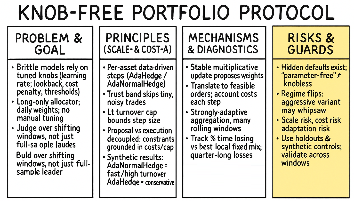
And here is where regime breaks come into action. This is the sudden change in loss geometry, volatility, and asset correlation. This is the event that makes all your tuned parameters obsolete overnight. So how do we solve this? The answer is to build an allocator that can allocate on the simplex Δ without any hand-tuning. It must be scale-free (to handle vol changes), cost-aware (to handle turnover), and strongly-adaptive (to handle regime breaks).

The solution that the machine learning and quant world offers, as we’ll see, is to move away from classic Exponentiated Gradient or Online Newton Step and embrace scale-free Hedge updates (like AdaHedge) at the asset level. This allocator is then coupled with a lazy rebalancing mechanism and strongly-adaptive wrappers to create a system that is robust by construction, not by tuning. No learning rate search, no window selection, no brittle temperature. Just math that works.

Online Portfolio Selection without knobs

Let’s formalize this. We’re operating in the classic Online Portfolio Selection or OPS setting. This is a sequential decision problem.

At the start of each day t=1, …, T, we must choose a long-only weight vector w_t. This vector must live on the N-dimensional simplex, Δ^N, meaning all weights are non-negative and sum to one:

\(\mathbf{w}_t \in \Delta^N := \{ \mathbf{w} \ge 0, \sum_{i=1}^N w_i = 1 \}\)

At the end of the day, the market reveals a vector of log-returns, r_t ∈R^N

Our gross wealth, in log space, evolves as:

\(\text{Eq}_{t+1}^{\text{gross}} = \text{Eq}_t^{\text{gross}} + \langle \mathbf{w}_t, \mathbf{r}_t \rangle\)

This is the standard, frictionless world. But trading is not free. We must model transaction costs. The most realistic model for institutional trading is a proportional L1 turnover cost. The cost to trade is proportional to the absolute value of the change in your portfolio weights.

\(\text{cost}_t = \lambda \| \mathbf{w}_{t+1} - \mathbf{w}_t \|_1\)

Here, λ is the cost parameter (e.g., λ=0.0002 for 2 bps). The L1 norm is key. If you sell 10% of asset A to buy 10% of asset B, your L1 turnover is |-0.10| + |+0.10| = 0.20.

Our net log-wealth, the only thing that actually matters, is therefore:

\(\text{Eq}_{t+1}^{\text{net}} = \text{Eq}_t^{\text{net}} + \langle \mathbf{w}_t, \mathbf{r}_t \rangle - \text{cost}_t\)

Most OPS methods, like Exponentiated Gradient (EG) or Online Newton Step (ONS), propose an update based on the day’s losses. Let L_t,i = -r_t,i be the loss for asset i. The classic EG update is:

\(w_{t+1, i} \propto w_{t, i} \exp(-\eta \ell_{t, i})\)

And here it is: η. The learning rate. The knob.

This η is poison. It is scale-sensitive. If your typical losses L_t,i are around 0.01 (1%), an η=0.5 might be fine. If the market panics and losses jump to 0.10 (10%), your update term exp(-0.5 x 0.10) is tiny, but exp(-0.5 x -0.10) is huge. The allocator’s weights will fly around, becoming brittle and unpredictable. You’ll either over-trade or under-react.

The core idea is to remove η. We will replace it with a data-driven, per-asset normalizer that automatically adapts the step size based on the history of losses for that specific asset. This is the scale-free idea.

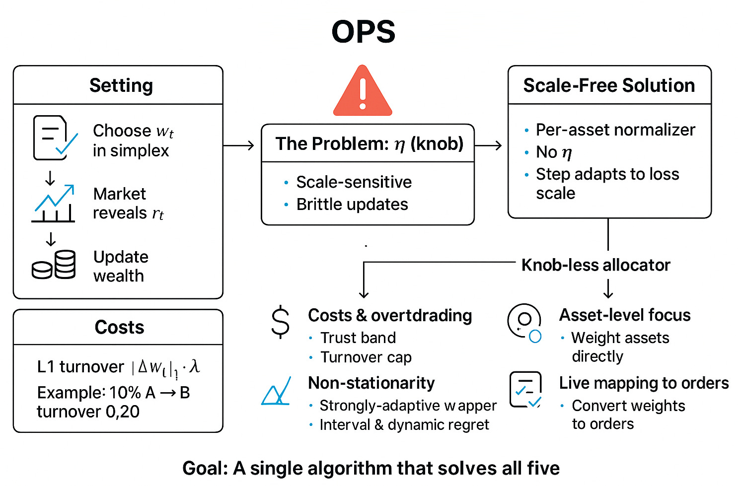
Building this knob-less allocator forces us to confront five major obstacles that are typically swept under the rug:

1. Costs and overtrading: We must not just model costs, we must constrain them. Even with a good update rule, a single large loss can cause a massive, costly portfolio jump. The algorithm must incorporate a trust band (to skip tiny, noisy rebalances) and a turnover cap (to prevent catastrophic, large rebalances).

2. Non-stationarity: As discussed, the world changes. Static regret (beating the best fixed portfolio) is insufficient. We need a system that performs well on interval regret (beating the best fixed portfolio on any sub-interval) and dynamic regret (adapting to shifting regimes). This requires a strongly-adaptive wrapper.

3. Numerical stability: Exponentials are dangerous. exp(1000) is inf. exp(-1000) is 0.0. An update like exp(-ηL_t) can easily overflow or underflow. The algorithm must be numerically stabilized, likely using the log-sum-exp trick, and must handle near-zero weights gracefully.

4. Asset-level vs. expert-level: Many online aggregation methods assume you have a set of “experts” (e.g., 10 different pre-built strategies) and you’re just weighting them. This is a cop-out. We are addressing the harder problem: allocating directly to the N assets themselves. Our experts are the assets.

5. Live mapping to orders: A vector w_t is not an order. A practical OPS algorithm must produce feasible, tradable orders. This means the weight vector must be translatable into orders that respect market freeze levels, safety ticks, partial fills, and other production realities.

Our goal is to build a single, coherent algorithm that solves all five of these problems simultaneously.

Mathematical framework

Here is the resolution. We will build our solution from the ground up, starting with a new mathematical framework.

Let’s be precise.

• Per-asset losses are:

  \(\ell_t = - \mathbf{r}_t \in \mathbb{R}^N\)

• The portfolio’s loss (ignoring costs for a moment) is:

  \(\ell_t(\mathbf{w}_t) = \langle \mathbf{w}_t, \ell_t \rangle\)

The entire field of Online Convex Optimization, from which OPS is derived, is built around the concept of regret. Regret is the difference between your algorithm’s cumulative loss and the loss of some optimal comparator in hindsight. The game is to minimize this regret. Check the previous article to know more about that:

[WITH CODE] Optimization: Adaptive regret for regime-shifting markets

The key perspective shift is in what you choose as your comparator.

1. Static regret → This is the classic definition. The comparator is the single best fixed-weight portfolio over the entire history T.

   \(R_T^{\text{stat}} = \sum_{t=1}^T \ell_t(\mathbf{w}_t) - \min_{\mathbf{w}^* \in \Delta^N} \sum_{t=1}^T \ell_t(\mathbf{w}^*)\)

   Algorithms like EG can guarantee a regret of

   \(R_T^{\text{stat}} = \mathcal{O}(\sqrt{T \log N})\)

   assuming bounded losses. This is a nice theoretical result, but practically useless. It tells you nothing about performance during a regime change.

2. Interval regret → This is much stronger. We want to be competitive over all possible contiguous windows [s, e] from 1 ≤ s ≤ e ≤ T.

   \(R_{s,e} = \sum_{t=s}^e \ell_t(\mathbf{w}_t) - \min_{\mathbf{w}^* \in \Delta^N} \sum_{t=s}^e \ell_t(\mathbf{w}^*)\)

   We want to ensure that max_{1 ≤ s ≤ e ≤ T} R_s,e is small. This is a much harder benchmark and is what diagnostics should focus on.

3. Dynamic (shifting) regret → This is the most realistic comparator. We compare our algorithm to the best sequence of portfolios w^*₁, …, w^*_T, but we penalize that sequence for its own turnover.

   \(R_T^{\text{dyn}} = \sum_{t=1}^T \ell_t(\mathbf{w}_t) - \min_{\mathbf{w}_1^*, \dots, \mathbf{w}_T^* \in \Delta^N} \left( \sum_{t=1}^T \ell_t(\mathbf{w}_t^*) + C \sum_{t=1}^{T-1} \|\mathbf{w}_{t+1}^* - \mathbf{w}_t^*\|_1 \right)\)

   This captures the essence of adapting to S different regimes.

Our algorithm won’t explicitly optimize for all of these, but its scale-free nature will give it strong performance on all three, especially interval and dynamic regret.

AdaHedge and AdaNormalHedge