[WITH CODE] Options: Iron Condor Strategy

Strategies with options

---

Table of contents:

1. Introduction.

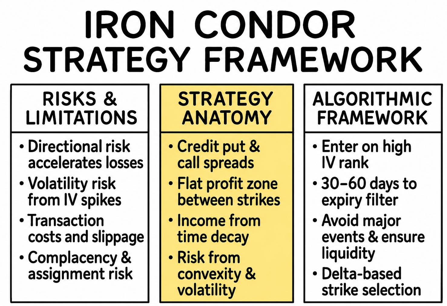
2. Risks and limitations of the strategy.

3. The mathematical anatomy of the Iron Condor.

4. The Greeks.

5. Beyond the payoff diagram.

6. Trading Vega.

7. Algorithmic entry and strike selection logic.

---

Introduction

The iron condor’s appeal is statistically seductive: a high-probability, defined-risk structure promising steady income from time decay and volatility erosion. Yet beneath its deceptively flat payoff profile lies a quantitatively intricate reality—one where theoretical win rates often mask a negative expected value. This isn’t a flaw in the strategy itself, but a consequence of its dynamic risk profile and the operational friction inherent in live trading.

The core paradox is straightforward: a position boasting a 90% theoretical probability of profit (POP) can systematically underperform due to three quantifiable forces. First, negative gamma accelerates losses nonlinearly as the underlying breaches short strikes, transforming modest moves into structural damage. Second, negative vega exposes the position to volatility shocks—where a spike in implied volatility alone can erase gains without price breaching strikes. Third, transaction costs—bid-ask spreads, multi-leg slippage, and execution latency—systematically erode the edge, particularly in high-turnover regimes. Together, these factors invert the strategy’s apparent statistical edge: frequent small wins are overwhelmed by infrequent but severe losses, yielding a negative Sharpe ratio despite the comforting 90% POP.

This isn’t a retail-trader cautionary tale. For systematic traders, the challenge is structural: How do you isolate and neutralize the latent risks that backtests obscure? Static payoff diagrams ignore the path-dependent dynamics of the Greeks; naive strike selection ignores volatility surface curvature; and "set-and-forget" execution ignores real-world market microstructure. The solution demands a rigorous, adaptive framework—one that treats the iron condor not as a static trade, but as a dynamic system requiring continuous recalibration of risk exposure, strike selection, and adjustment triggers.

Today we dissect that framework. We move beyond the oversimplified narrative of selling volatility to address the quantifiable mechanics of this strategy. For deeper insights check this:

Iron Condor Strategy

718KB ∙ PDF file

Download

Download

The goal isn’t to promise consistent profits, but to define the precise conditions under which the strategy’s statistical edge could survive the market. However, in future articles we will see that there are many more latent pitfalls due to the Black Scholes model and that they will be addressed with an arbitrage-aware framework.

Risks and limitations of the strategy

The primary risk of the Iron Condor strategy is its asymmetric risk/reward profile: you accept the low probability of a potentially large loss in exchange for the high probability of a small, limited gain.

1. Market-related risks:

   1. While the strategy profits from a sideways market, a sharp, significant price movement in either direction can cause substantial losses. Due to the position's negative gamma—direction risk—these losses accelerate the further the price moves against you. A small move might be manageable, but a fast, large move can quickly erase the initial premium and lead to the maximum loss.

   2. An Iron Condor is a short volatility strategy—Vega risk. This means it profits when implied volatility (IV) decreases or stays the same. If market fear spikes and implied volatility rises suddenly, the value of your position will decrease, creating a loss even if the underlying price hasn't breached your short strikes.

2. Strategy-specific risks & limitations:

   1. Your maximum profit is always capped at the net credit you received when you opened the trade. You can never make more than this initial amount, no matter how perfectly the trade works out.

   2. Typically, the maximum potential loss on an Iron Condor is significantly greater than the maximum potential profit. For example, you might risk $850 to make a maximum of $150. This means one max-loss trade can wipe out the gains from five or more winning trades.

   3. The high probability and defined risk nature can make traders complacent. While the maximum loss is defined, it is often a substantial amount of capital. A high win rate does not guarantee long-term profitability if the few losing trades are not managed correctly.

   4. If you are trading American-style options—like those on most individual stocks—the person who bought the options from you can exercise their right to assign you shares at any time before expiration. This can force you into an unexpected stock position (either long or short) and disrupt your strategy—assignment risk.

The mathematical anatomy of the Iron Condor

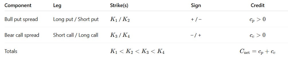
Before we can automate, we must first define. The Iron Condor is a four-legged options strategy composed of two distinct vertical spreads: a bear call spread and a cull put spread. The key is that both spreads are sold, making it a net credit strategy, and they are centered around the current price of the underlying asset, creating a market-neutral stance.

Positions and notations

Let's define the elements that translate the relationships of the strategy into mathematical equations.

1. Structure:

   Let the underlying price at expiry be S_T​. Choose strikes

   \(K_1<K_2<K_3<K_4,\)

   with the trade typically centered so that the entry spot S₀​ (and the expected S_T​) lie between K₂​ and K₃​.

   The Iron Condor is the simultaneous sale of:

   • A bull put spread: short put at K₂​, long put at K₁​;

   • A bear call spread: short call at K₃​, long call at K₄​.

   Let the credits received be

   \(c_p=\text{credit from put spread},\qquad c_c=\text{credit from call spread},\qquad C_{\text{net}} = c_p+c_c.\)

   Now we define wing widths

   \(W_{\text{put}}=K_2-K_1,\qquad W_{\text{call}}=K_4-K_3.\)

   No‑arbitrage implies 0≤c_p​≤W_put​ and 0≤c_c≤W_call, hence

   \(0\le C_{\text{net}}\le W_{\text{put}}+W_{\text{call}}.\)

2. Option payoffs at expiry:

   For any strike K,

   \(C(S_T,K)=\max(0,S_T-K),\qquad P(S_T,K)=\max(0,K-S_T),\)

   and a short position is the negative of the corresponding long payoff.

   The four legs therefore contribute:

   \(\begin{aligned} \text{Long }K_1\text{ put: } & +\, (K_1-S_T)^+,\\ \text{Short }K_2\text{ put: } & -\, (K_2-S_T)^+,\\ \text{Short }K_3\text{ call: }& -\, (S_T-K_3)^+,\\ \text{Long }K_4\text{ call: }& +\, (S_T-K_4)^+. \end{aligned}\)

   Adding the entry credit C_net​ gives the expiry payoff—profit, excluding financing:

   \(\boxed{ \Pi(S_T)= C_{\text{net}} +(K_1-S_T)^+-(K_2-S_T)^+ -(S_T-K_3)^+ + (S_T-K_4)^+ . }\)

   Equivalently,

   \(\Pi(S_T)= C_{\text{net}} -\big[(K_2-S_T)^+-(K_1-S_T)^+\big] -\big[(S_T-K_3)^+-(S_T-K_4)^+\big],\)

   i.e., minus the intrinsic of each short spread plus the credit.

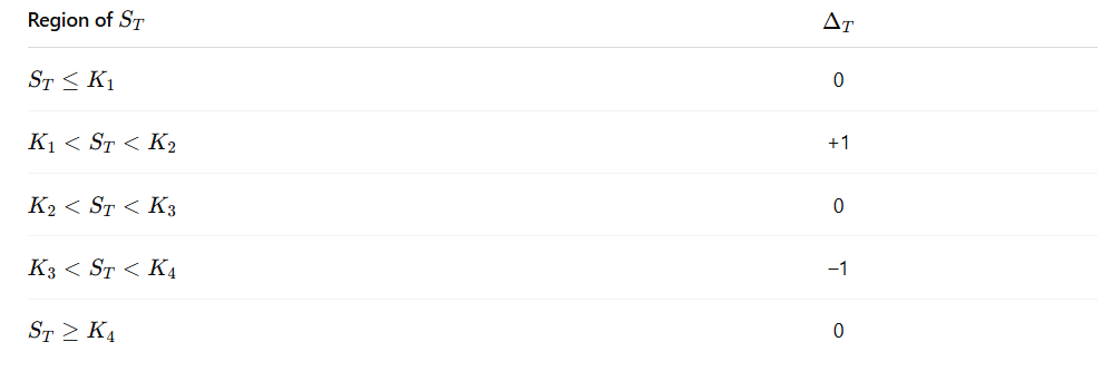
3. Piecewise form and interpretation of the five regions:

   \(\Pi(S_T)= \begin{cases} \displaystyle C_{\text{net}}+K_1-K_2 = C_{\text{net}}-W_{\text{put}}, & S_T\le K_1 \quad \text{(max loss floor, downside)},\\[6pt] \displaystyle C_{\text{net}}-K_2+S_T, & K_1<S_T\le K_2 \quad \text{(loss zone, slope }+1),\\[6pt] \displaystyle C_{\text{net}}, & K_2<S_T<K_3 \quad \text{(max‑profit plateau)},\\[6pt] \displaystyle C_{\text{net}}+K_3-S_T, & K_3\le S_T<K_4 \quad \text{(loss zone, slope }-1),\\[6pt] \displaystyle C_{\text{net}}+K_3-K_4 = C_{\text{net}}-W_{\text{call}}, & S_T\ge K_4 \quad \text{(max loss floor, upside)}. \end{cases}\)

   Why these shapes?

   • Tails are flat when S_T≤K₁ (deep downside), both puts are ITM by the same amount; the S_T​ terms cancel and you realize the put‑spread loss W_put offset by the credit. Symmetrically, for S_T≥K₄​ the calls are both ITM and you realize C_net−W_call​.

   • We have two sloped zones:

     • K₁<S_T≤K₂: only the short K₂​ put is ITM, so each $1 rise in S_T​ reduces that intrinsic value by $1; payoff slope +1.

     • K₃≤S_T<K₄​: only the short K₃​ call is ITM; each $1 rise in S_T​ increases loss by $1; slope −1.

   • The center remains flat if K₂<S_T<K₃​: all options OTM; payoff equals the entry credit.

   At expiry the position delta (slope of Π) is 0, +1, 0, −1, across the five regions; gamma is zero except at the kinks K₁, K₂, K₃, K₄​.

4. How do we calculate the extremes?

   • The extremes are immediate. The maximum payoff occurs on the plateau:

     \(\boxed{\Pi_{\max}=C_{\text{net}}} \quad \text{for } K_2<S_T<K_3.\)

   • The minimum payoff is the lower of the two floors:

     \(\boxed{\Pi_{\min}=C_{\text{net}}-\max\!\big(W_{\text{put}},W_{\text{call}}\big)}.\)

   • So the maximum loss in cash is:

     \(\boxed{L_{\max}=\max\!\big(W_{\text{put}},W_{\text{call}}\big)-C_{\text{net}}.}\)

     Per side, the losses are:

     \(L_{\text{down}}=W_{\text{put}}-c_p,\qquad L_{\text{up}} =W_{\text{call}}-c_c,\qquad L_{\max}=\max(L_{\text{down}},L_{\text{up}}).\)

   • Symmetric wings are created by W_put=W_call=W:

     \(\Pi_{\min}=C_{\text{net}}-W,\qquad L_{\max}=W-C_{\text{net}}.\)

5. How do we calclulate the break-even levels?

   Set Π(S_T)=0 on the sloped segments:

   \(\begin{aligned} 0 &= C_{\text{net}}-K_2+S_T &&\Rightarrow& \boxed{S_T^{\text{BE-}}=K_2-C_{\text{net}}}\in[K_1,K_2],\\[4pt] 0 &= C_{\text{net}}+K_3-S_T &&\Rightarrow& \boxed{S_T^{\text{BE+}}=K_3+C_{\text{net}}}\in[K_3,K_4]. \end{aligned}\)

   A larger C_net​ widens the break‑even interval and raises both floors, but given c_p≤W_put​ and c_c≤W_call​, the loss on each side remains non‑negative.

It is more simple than the math explained before. Let's visualize this step by step. The first code snippet defines a function to calculate the Iron Condor payoff.

import numpy as np
import matplotlib.pyplot as plt

def iron_condor_payoff(s_t, k1, k2, k3, k4, c_net):
    """
    Calculates the P/L of an Iron Condor at expiration.

    Args:
        s_t (np.array): Array of underlying prices at expiration.
        k1 (float): Long put strike.
        k2 (float): Short put strike.
        k3 (float): Short call strike.
        k4 (float): Long call strike.
        c_net (float): Net credit received for the position.

    Returns:
        np.array: P/L for each underlying price.
    """
    long_put_payoff = np.maximum(0, k1 - s_t)
    short_put_payoff = -np.maximum(0, k2 - s_t)
    short_call_payoff = -np.maximum(0, s_t - k3)
    long_call_payoff = np.maximum(0, s_t - k4)
    
    total_payoff = c_net + long_put_payoff + short_put_payoff + short_call_payoff + long_call_payoff
    return total_payoff

# --- Strategy Parameters ---
# Let's assume the underlying is trading at $100.
K1_put_long = 85.0
K2_put_short = 90.0
K3_call_short = 110.0
K4_call_long = 115.0
Net_Credit = 1.50 # Example credit received in $

# --- Plotting ---
S_T = np.arange(75, 125, 0.1) # Range of underlying prices at expiration
payoff = iron_condor_payoff(S_T, K1_put_long, K2_put_short, K3_call_short, K4_call_long, Net_Credit)

# Calculate key points
max_profit = Net_Credit
max_loss = Net_Credit - (K2_put_short - K1_put_long)
breakeven_down = K2_put_short - Net_Credit
breakeven_up = K3_call_short + Net_Credit

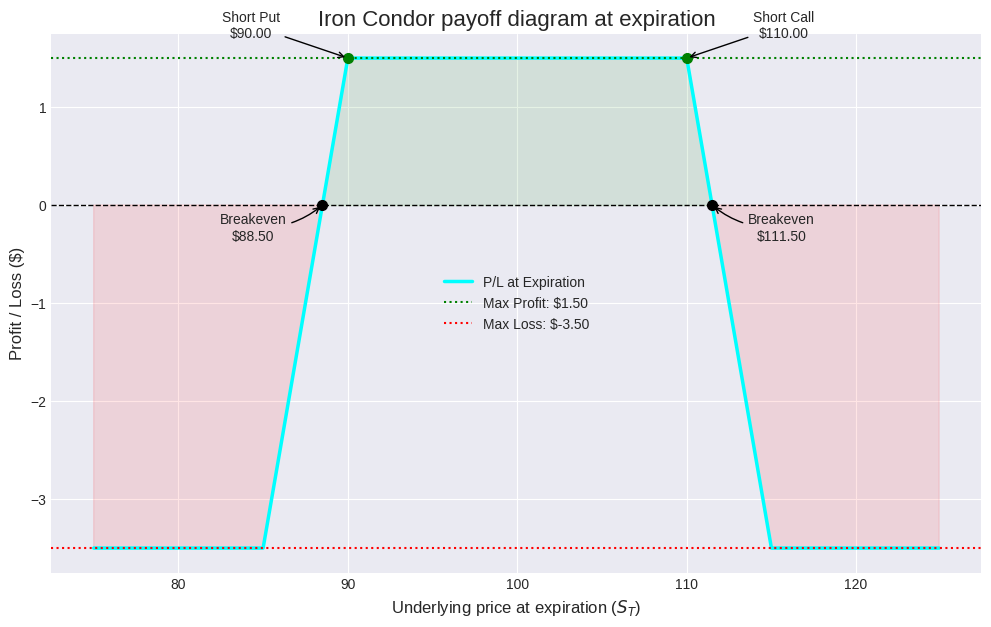
This plot is the classic, static representation. It is essential, but it tells us nothing about the expiration. The next part will explore the dynamics of the position before this final payoff is realized.

The Greeks

The payoff diagram is a static snapshot at a single point in time: expiration. To manage the strategy effectively, a quant must understand the position's real-time risk profile. This is where the Greeks come in. They are the partial derivatives of the option's price with respect to various market variables.

The aggregate Greeks of the four legs define its behavior. Where the price is simply the sum of the prices of its components: V_condor=P(K₁)−P(K₂)−C(K₃)+C(K₄)

Where P(K) and C(K) are the Black-Scholes prices for put and call options with strike K. The Greeks of the Condor are therefore the sum of the Greeks of the individual options.

\(Greek_{condor}​=Greek_{P(K_1​)}​−Greek_{P(K_2​)}​−Greek_{C(K_3​)}​+Greek_{C(K_4​)}​\)

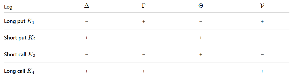
We now examine the key Greeks for this strategy:

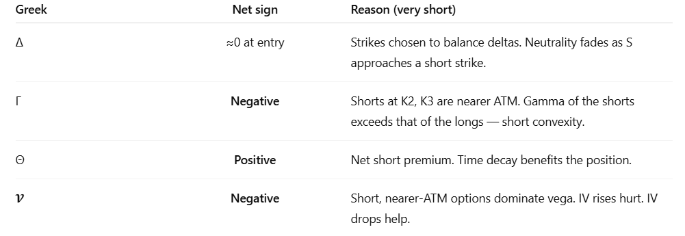
1. Delta → Δ=∂V/∂S:

   Delta measures the rate of change of the option's price with respect to a $1 change in the underlying asset's price.

   • Long put (K₁): Negative Delta.

   • Short put (K₂): Positive Delta.

   • Short call (K₃): Negative Delta.

   • Long call (K₄): Positive Delta.

   When a Condor is initiated at-the-money, the strikes are chosen to balance these positive and negative deltas, creating a delta-neutral position. This means, for small movements in the underlying, the position's value shouldn't change much. However, as the price moves towards one of the short strikes, this neutrality is lost.

2. Gamma → Γ=∂²V/∂S²:

   Gamma measures the rate of change of Delta. It's the convexity of the position.

   • Long options (puts or calls): Positive Gamma.

   • Short options (puts or calls): Negative Gamma.

   The Iron Condor is a net short option position (2 short, 2 long, but the shorts are closer to the money and have higher gamma). This results in net negative Gamma. This is the single most important risk factor. Negative gamma means that as the underlying moves against you, your Delta becomes more adverse. If the price rises, your Delta becomes more negative. If the price falls, your Delta becomes more positive. You are short convexity, and losses accelerate.

3. Theta → Θ=-∂V/∂t:

   Theta measures the rate of change of the option's price with respect to the passage of time (time decay).

   • Long options: Negative Theta (they lose value as time passes).

   • Short options: Positive Theta (they gain value as time passes).

   The Iron Condor is a net short premium strategy, resulting in net positive Theta. This is the profit engine of the strategy. Every day that passes, assuming the underlying price and volatility remain constant, the position should make money from time decay. The core trade-off of the Iron Condor is this: You accept negative Gamma risk in exchange for positive Theta profit.

4. Vega → V=∂V/∂σ:

   Vega measures sensitivity to a 1% change in implied volatility (sigma).

   • Long Options: Positive Vega.

   • Short Options: Negative Vega.

   Since the short options (K₂, K₃) are closer to the money, they have higher Vega than the far out-of-the-money long options (K₁, K₄). This results in net negative Vega. A rise in implied volatility will hurt the position, while a fall in implied volatility will help it. This is why Iron Condors are often initiated in high implied volatility environments, with the expectation that IV will revert to its mean.

We can summarize this information in the next tables:

Per‑leg Greek signs

Net exposures

Expiry delta by region

Much better. Okay! For this example we will use a library like py_vollib to calculate the Black-Scholes price and Greeks for each leg and then aggregate them.

#!pip install py_vollib
import py_vollib.black_scholes.greeks.analytical as greeks
from py_vollib.black_scholes import black_scholes as bs

def calculate_condor_greeks(s, k1, k2, k3, k4, t, r, sigma):
    """
    Calculates the aggregated Greeks for an Iron Condor.
    
    Args:
        s (float): Current underlying price.
        k1, k2, k3, k4 (float): Strike prices.
        t (float): Time to expiration in years.
        r (float): Risk-free interest rate.
        sigma (float): Implied volatility.
        
    Returns:
        dict: A dictionary containing the position's delta, gamma, theta, and vega.
    """
    # Calculate greeks for each leg
    delta1 = greeks.delta('p', s, k1, t, r, sigma)
    delta2 = -greeks.delta('p', s, k2, t, r, sigma)
    delta3 = -greeks.delta('c', s, k3, t, r, sigma)
    delta4 = greeks.delta('c', s, k4, t, r, sigma)
    
    gamma1 = greeks.gamma('p', s, k1, t, r, sigma)
    gamma2 = -greeks.gamma('p', s, k2, t, r, sigma)
    gamma3 = -greeks.gamma('c', s, k3, t, r, sigma)
    gamma4 = greeks.gamma('c', s, k4, t, r, sigma)

    theta1 = greeks.theta('p', s, k1, t, r, sigma) / 365.25
    theta2 = -greeks.theta('p', s, k2, t, r, sigma) / 365.25
    theta3 = -greeks.theta('c', s, k3, t, r, sigma) / 365.25
    theta4 = greeks.theta('c', s, k4, t, r, sigma) / 365.25

    vega1 = greeks.vega('p', s, k1, t, r, sigma) / 100
    vega2 = -greeks.vega('p', s, k2, t, r, sigma) / 100
    vega3 = -greeks.vega('c', s, k3, t, r, sigma) / 100
    vega4 = greeks.vega('c', s, k4, t, r, sigma) / 100
    
    # Aggregate greeks
    total_delta = delta1 + delta2 + delta3 + delta4
    total_gamma = gamma1 + gamma2 + gamma3 + gamma4
    total_theta = theta1 + theta2 + theta3 + theta4
    total_vega = vega1 + vega2 + vega3 + vega4
    
    return {'delta': total_delta, 'gamma': total_gamma, 'theta': total_theta, 'vega': total_vega}

# --- Parameters for Greek Calculation ---
S_range = np.arange(80, 121, 1) # Price range to analyze
T = 45.0 / 365.25 # 45 days to expiration
R = 0.05 # 5% risk-free rate
SIGMA = 0.20 # 20% implied volatility

# Use the same strikes as before
K1, K2, K3, K4 = 85, 90, 110, 115

# Calculate greeks across the price range
condor_greeks_list = [calculate_condor_greeks(s, K1, K2, K3, K4, T, R, SIGMA) for s in S_range]

# Extract individual greeks for plotting
deltas = [g['delta'] for g in condor_greeks_list]
gammas = [g['gamma'] for g in condor_greeks_list]
thetas = [g['theta'] for g in condor_greeks_list]
vegas = [g['vega'] for g in condor_greeks_list]

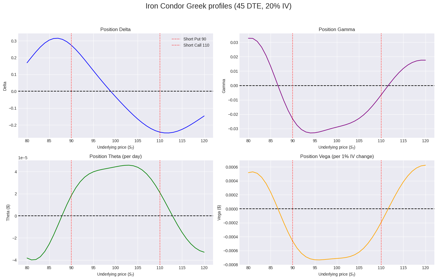
The plots reveal the dynamic nature of the risk.

1. Delta is near zero between the short strikes but quickly becomes positive below K₂ and negative above K₃. This is the directional risk.

2. Gamma is negative across the board, but most strongly negative near the short strikes. This is the acceleration risk.

3. Theta is positive, peaking between the strikes. This is the income.

4. Vega is negative, also most strongly near the strikes. This is the volatility risk.

An algorithmic system must monitor these Greeks in real-time. A rule might be: If absolute position Delta exceeds 0.10, trigger an adjustment, or If the underlying price moves to a point where Gamma is below -0.05, raise an alert.

Beyond the payoff diagram

The most common mistake traders make with Iron Condors is conflating a high POP with a positive Expected Value. You might advertise a trade with a 90% chance of success, which sounds fantastic. However, if the 10% of losing trades lose, on average, more than 9 times the amount gained from the winners, the strategy has a negative EV and is a long-term loser.

\(EV=(P(Win)×Avg. Win)−(P(Loss)×Avg. Loss)\)

For an Iron Condor, the Avg. Win is capped at the net credit received. The Avg. Loss can be significantly larger. A quantitative approach demands that we move beyond the simple POP and analyze the full probability distribution of outcomes.

To calculate these probabilities, we need a model for the future distribution of the underlying asset's price. The standard model in finance is that asset prices follow a Geometric Brownian Motion, which means that log-returns are normally distributed. Consequently, the price at expiration, S_T, follows a log-normal distribution.

The parameters for this distribution are:

1. Current Price: S_T.

2. Time to Expiration: T.

3. Drift: mu (often assumed to be the risk-free rate, r, in the risk-neutral world).

4. Volatility: sigma (the implied volatility derived from option prices).

The expected price at expiration is E[S_T]=S_Te^mu·T. The standard deviation of the log price is σ√T

The POP is the probability that the underlying price S_T will finish between the breakeven points at expiration.

• Breakeven down: K_BE, down=K₂ −C_net

• Breakeven up: K_BE, up=K₃+C_net

So, we need to calculate P(K_BE,down < S_T< K_BE,up). Using the log-normal assumption, this can be calculated from the cumulative distribution function (CDF) of the normal distribution.

Let

\(x = \ln\!\frac{S_T}{S_t}.\)

We assume

\(x \sim \mathcal{N}\!\Bigl(\bigl(\mu - \tfrac12\sigma^2\bigr)T,\;\sigma^2\,T\Bigr).\)

Then the probability of profit is modeled by:

\(\mathrm{POP} = \mathbb{P}\!\Bigl(\substack{\ln\!\frac{K_{\mathrm{BE,down}}}{S_t} < x < \ln\!\frac{K_{\mathrm{BE,up}}}{S_t}}\Bigr).\)

Let's write Python code to calculate the POP and, more importantly, to visualize the entire P/L distribution. This gives a much richer view of the risk-reward tradeoff than a single EV number.

import scipy.stats as stats

def analyze_condor_probabilities(s_t, k1, k2, k3, k4, c_net, t, r, sigma):
    """
    Analyzes the probabilistic outcomes of an Iron Condor.
    
    Returns:
        dict: Containing POP, EV, and data for plotting.
    """
    # Breakeven points
    breakeven_down = k2 - c_net
    breakeven_up = k3 + c_net
    
    # Lognormal distribution parameters for S_T
    mu = (r - 0.5 * sigma**2) * t
    std_dev = sigma * np.sqrt(t)
    
    # Calculate Probability of Profit (POP)
    z_down = (np.log(breakeven_down / s_t) - mu) / std_dev
    z_up = (np.log(breakeven_up / s_t) - mu) / std_dev
    pop = stats.norm.cdf(z_up) - stats.norm.cdf(z_down)
    
    # Simulate a large number of outcomes for EV and plotting
    num_simulations = 250000
    # S_T = s_t * np.exp(mu + std_dev * np.random.randn(num_simulations)) # Lognormal sample
    # Using stats.lognorm.rvs for clarity
    lognorm_dist = stats.lognorm(s=std_dev, scale=np.exp(mu) * s_t)
    simulated_s_t = lognorm_dist.rvs(size=num_simulations)

    # Calculate P/L for each simulated outcome
    simulated_pl = iron_condor_payoff(simulated_s_t, k1, k2, k3, k4, c_net)
    
    expected_value = np.mean(simulated_pl)
    
    return {
        'pop': pop,
        'expected_value': expected_value,
        'simulated_s_t': simulated_s_t,
        'simulated_pl': simulated_pl,
        'dist': lognorm_dist
    }

# --- Parameters ---
S_t = 100.0
K1, K2, K3, K4 = 85, 90, 110, 115
C_net = 1.50
T = 45.0 / 365.25
R = 0.05
SIGMA = 0.20 # 20% IV

# --- Run Analysis ---
analysis = analyze_condor_probabilities(S_t, K1, K2, K3, K4, C_net, T, R, SIGMA)

print(f"Probability of Profit (POP): {analysis['pop']:.2%}")
print(f"Expected Value (EV) from Simulation: ${analysis['expected_value']:.4f}")

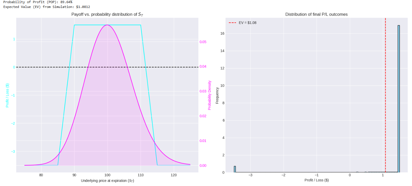
This analysis provides a much clearer picture.

• The first plot shows why the POP is high: the bulk of the probability distribution for the final price lies squarely within the profitable range of the condor. However, it also shows the tails of the distribution extending into the max loss zones.

• The second plot, the P/L distribution, is the most sobering. It typically shows a large spike at the max profit value and smaller, but significant, frequencies in the loss regions. The negative skew is apparent: the potential for large losses pulls the mean (the Expected Value) down. In this specific example, the EV might be positive, but a small increase in volatility or a wider spread could easily turn it negative, even with a high POP.

An algorithmic system can run this analysis before placing any trade, refusing to enter positions with a negative EV, regardless of the POP. This is a fundamental quantitative filter.

Trading Vega

The Iron Condor is, at its heart, a short volatility strategy. Its profitability is intrinsically linked to the behavior of implied volatility (IV). As shown by its negative Vega, the position benefits when IV decreases and suffers when IV increases. A successful algorithmic approach to Iron Condors is therefore less about predicting price direction and more about correctly forecasting the direction of volatility.

This is the cornerstone of volatility trading:

1. Implied Volatility (IV): The market's forecast of future volatility, as implied by current option prices. It's the sigma we plug into the Black-Scholes model.

2. Realized (or historical) Volatility (HV): The actual volatility of the underlying asset as measured over a historical period.

Systematic profits can be made by exploiting the Volatility Risk Premium (VRP). This is the well-documented empirical phenomenon where IV, on average, tends to be higher than the subsequent HV. Option sellers—like those selling Iron Condors—are essentially collecting this premium as compensation for taking on the risk of volatility spikes—gamma risk.

An algorithm's primary signal should be based on identifying when this premium is abnormally high. This is done using IV Rank (IVR) or IV Percentile (IVP).

1. IV Rank: Measures where the current IV lies in relation to its high and low over a lookback period (e.g., one year). IVR = (Current IV - 52wk Low IV) / (52wk High IV - 52wk Low IV). An IVR of 90% means the current IV is in the top 10% of its annual range.

2. IV Percentile: Measures what percentage of days over the lookback period had a lower IV than the current IV.

The trading thesis is simple: Sell premium when IV is high (high IVR/IVP), and avoid it or buy premium when IV is low.

Volatility is not constant across all strike prices for a given expiration. This variation is known as the volatility smile or skew.

• Smile: OTM puts and calls have higher IV than ATM options.

• Skew: OTM puts have a significantly higher IV than corresponding OTM calls. This reflects the market's higher demand for downside protection (puts), leading to a fear premium.

A quant must account for the skew when selecting strikes. Choosing strikes based on a fixed number of points from the current price is naive. A better method is to select strikes based on a constant Delta, for instance, selling the 16-delta put and the 16-delta call. This standardizes the initial probability of a strike being touched and automatically adjusts the width of the position based on the market's own pricing of risk.

In a real system, you would connect to a data provider API—like Interactive Brokers, TDAmeritrade, or a dedicated data vendor. For this example, let's create a pseudo-code structure for an algorithm that scans a list of underlyings and identifies high-IV environments suitable for an Iron Condor.

import pandas as pd

# This is a MOCK function. In reality, this would make an API call.
def get_option_chain_and_iv(ticker):
    """
    MOCK FUNCTION: Simulates fetching option chain data and IV metrics.
    In a real implementation, this connects to a broker/data API.
    """
    print(f"Fetching data for {ticker}...")
    # Simulate data for a stock trading at $200
    if ticker == "SPY":
        return {
            "underlying_price": 450.0,
            "iv_current": 0.18, # 18%
            "iv_52wk_low": 0.12, # 12%
            "iv_52wk_high": 0.35, # 35%
            # A simplified options chain for a specific expiration (e.g., 45 DTE)
            "chain": pd.DataFrame({
                'strike': [420, 425, 430, 460, 465, 470],
                'type': ['put', 'put', 'put', 'call', 'call', 'call'],
                'delta': [-0.25, -0.35, -0.45, 0.33, 0.24, 0.16],
                'iv': [0.21, 0.20, 0.19, 0.17, 0.16, 0.15] # Example of skew
            })
        }
    else: # Simulate a high-IV stock
        return {
            "underlying_price": 150.0,
            "iv_current": 0.65, # 65%
            "iv_52wk_low": 0.30, # 30%
            "iv_52wk_high": 0.70, # 70%
            "chain": pd.DataFrame({
                'strike': [120, 125, 130, 170, 175, 180],
                'type': ['put', 'put', 'put', 'call', 'call', 'call'],
                'delta': [-0.16, -0.22, -0.28, 0.27, 0.21, 0.15],
                'iv': [0.69, 0.67, 0.66, 0.64, 0.63, 0.62]
            })
        }

def find_high_iv_candidates(ticker_list, min_iv_rank=70):
    """
    Scans a list of tickers to find candidates for selling premium.
    """
    candidates = []
    for ticker in ticker_list:
        data = get_option_chain_and_iv(ticker)
        if not data:
            continue
            
        iv_high = data['iv_52wk_high']
        iv_low = data['iv_52wk_low']
        iv_current = data['iv_current']
        
        # Avoid division by zero if high and low are the same
        if (iv_high - iv_low) == 0:
            iv_rank = 0
        else:
            iv_rank = (iv_current - iv_low) / (iv_high - iv_low) * 100
            
        print(f"--- Ticker: {ticker} ---")
        print(f"Current IV: {iv_current:.2%}")
        print(f"IV Rank: {iv_rank:.1f}%")
        
        if iv_rank >= min_iv_rank:
            print(f"STATUS: CANDIDATE FOUND! IV Rank is above {min_iv_rank}%.\n")
            candidates.append({'ticker': ticker, 'data': data})
        else:
            print(f"STATUS: Pass. IV Rank is too low.\n")
    return candidates

# --- Run the Scanner ---
tickers_to_scan = ["SPY", "TSLA"] # A low IV and a high IV example
potential_trades = find_high_iv_candidates(tickers_to_scan, min_iv_rank=50)

if potential_trades:
    print("\n--- Final List of High IV Candidates ---")
    for trade in potential_trades:
        print(trade['ticker'])

This snippet demonstrates the first step in the algorithmic funnel: filtering the entire universe of possible trades down to a manageable list of candidates that meet the primary condition for selling volatility. The next step is to select the exact strikes for these candidates.

Algorithmic entry and strike selection logic

Once a suitable high-IV underlying is identified, the algorithm must execute the core logic of constructing the Iron Condor. This involves defining precise, non-ambiguous rules for timing and strike selection.

1. Entry criteria:

   A robust entry signal is a confluence of several factors. Relying on a single metric is fragile. A typical set of entry rules for an automated system would be:

   1. Volatility filter: IV_Rank >= 70. This ensures we are selling premium when it is rich.

   2. Expiration cycle filter: 30 <= Days_to_Expiration <= 60. This is often considered the sweet spot. Shorter DTEs have rapid Theta decay but also extreme Gamma risk. Longer DTEs are slower and less capital efficient.

   3. Market state filter (Optional): Avoid entering new positions if the broad market is in a state of extreme panic (e.g., VIX > 40) or if there is a major known event (e.g., earnings announcement, FOMC meeting) before expiration. This helps to filter out non-statistical risks.

   4. Liquidity filter: Ensure the chosen options have tight bid-ask spreads and sufficient open interest to allow for easy entry and exit. An illiquid option can lead to massive slippage, destroying the trade's edge.

2. Strike selection:

   This is one of the most critical parameters. The goal is to set the short strikes far enough away that the probability of being breached is low, but close enough to collect a meaningful premium.

   1. Method 1: Standard deviations (the old way):

      One simple heuristic is to estimate the expected price move over your holding period by

      \(\text{Expected move} \;\approx\; S_t \;\times\;\sigma\;\times\sqrt{\frac{T}{365}},\)

      and then set your short strikes just outside that band—say one volatility‑sigma away from spot. It’s better than picking strikes at random, but it completely ignores the term structure and skew of implied vol, both of which can substantially change where the true risk lies.

   2. Method 2: Option delta (the professional's way):

      Delta can be used as a rough proxy for the probability of an option expiring in-the-money. A 16-delta option has, roughly, a 16% chance of expiring ITM.

      A common systematic approach is:

      1. Sell the short strikes: Identify the put option with a delta closest to -0.16 and the call option with a delta closest to +0.16. These become the short legs (K₂ and K₃).

      2. Buy the long strikes: Buy the protective wings a fixed distance away. For example, if trading an index like SPX, one might set the wings 10 or 20 points further out. The width of the wings (W=K₂ −K₁=K₄−K₃) directly determines the maximum risk and the capital requirement for the trade. The choice of wing width is a trade-off between the premium collected (a wider spread collects a slightly higher credit) and the risk-reward ratio. A common rule is to aim for a net credit that is roughly 1/3 of the wing width.

Let's translate this logic into a function. This function would take the data from our scanner and construct the final trade.

import pandas as pd

def construct_delta_based_condor(symbol, chain, target_delta=0.16, wing_width=10):
    """
    Constructs an Iron Condor based on target delta for the short strikes.

    Args:
        symbol (str): Underlying ticker symbol.
        chain  (pd.DataFrame): Option chain with columns ['type','strike','delta', …].
        target_delta (float): Absolute delta for the short strikes.
        wing_width   (float): Wing‐width in strike units.

    Returns:
        dict or None: Four‐leg Condor definition, or None if invalid.
    """
    # Split puts and calls
    puts  = chain[chain['type'] == 'put'].copy()
    calls = chain[chain['type'] == 'call'].copy()

    # Find the short put (|delta| closest to target_delta)
    puts['delta_dist'] = (puts['delta'].abs() - target_delta).abs()
    short_put = puts.sort_values('delta_dist').iloc[0]

    # Find the short call (delta closest to +target_delta)
    calls['delta_dist'] = (calls['delta'] - target_delta).abs()
    short_call = calls.sort_values('delta_dist').iloc[0]

    # Define strikes
    K2 = short_put['strike']   # short put
    K3 = short_call['strike']  # short call
    K1 = K2 - wing_width       # long put
    K4 = K3 + wing_width       # long call

    # Sanity check: strict ordering
    if not (K1 < K2 < K3 < K4):
        print(f"ERROR: strikes not strictly ordered: {K1}, {K2}, {K3}, {K4}")
        return None

    # Warn if long strikes missing
    available = set(chain['strike'])
    for K in (K1, K4):
        if K not in available:
            print(f"WARNING: strike {K} not found in chain; liquidity unknown")

    trade = {
        'underlying': symbol,
        'status':     'PENDING_EXECUTION',
        'legs': {
            'long_put':   {'strike': K1, 'action': 'BUY',  'delta': None},
            'short_put':  {'strike': K2, 'action': 'SELL', 'delta': short_put['delta']},
            'short_call': {'strike': K3, 'action': 'SELL', 'delta': short_call['delta']},
            'long_call':  {'strike': K4, 'action': 'BUY',  'delta': None},
        },
        'wing_width':   wing_width,
        'target_delta': target_delta,
    }

    print("\n--- Proposed Iron Condor Trade ---")
    print(f"Underlying:    {symbol}")
    print(f"Long Put  @ {K1}")
    print(f"Short Put @ {K2} (Δ={short_put['delta']:.2f})")
    print(f"Short Call@ {K3} (Δ={short_call['delta']:.2f})")
    print(f"Long Call @ {K4}")

    return trade

#---Run the example---
chain_df = pd.DataFrame([
        {'type':'put',  'strike':145, 'delta':-0.18},
        {'type':'put',  'strike':150, 'delta':-0.15},
        {'type':'call', 'strike':155, 'delta': 0.16},
        {'type':'call', 'strike':160, 'delta': 0.18},])

candidate = {'symbol':'TSLA', 'chain': chain_df}

final_trade_plan = construct_delta_based_condor(
    symbol       = candidate['symbol'],
    chain        = candidate['chain'],
    target_delta = 0.15,
    wing_width   = 5,)

if final_trade_plan:
  print("\nACTION: Send trade plan to execution handler.")

This systematic, rule-based approach removes emotional decision-making and ensures consistency. The parameters (target_delta, wing_width, DTE, IV_Rank) can be rigorously optimized.

Finally, let's run the complete code I've provided in the appendix below. Let's see what this does with fake data.

Pretty cool right!? All right, everyone! Fantastic work today! This wasn’t a simple strategy. The perception of the Iron Condor as a low-effort, "set and forget" source of income is a dangerous misconception. The path to successfully trading Iron Condors, especially in an algorithmic context, is paved with calculus, statistics, and code.

Time to power down and recharge. Keep questioning, keep exploring, keep that quant spirit alive! Stay quanty!🚀

---

👍🏻 If you liked the article and are interested in this topic, feel free to join our discussion group!

---

PS: What is the most critical part for you in a trading system?

Appendix

Full script:

!pip install py_vollib
import numpy as np
import pandas as pd
import matplotlib.pyplot as plt
import scipy.stats as stats
import py_vollib.black_scholes.greeks.analytical as greeks
from py_vollib.black_scholes import black_scholes

# Set plot style for better visuals
plt.style.use('seaborn-v0_8-darkgrid')

class IronCondorStrategy:
    """
    A framework for analyzing, constructing, and monitoring Iron Condor trades.
    
    This class encapsulates the logic for:
    1. Finding high implied volatility trade candidates.
    2. Constructing delta-neutral Iron Condors.
    3. Analyzing the trade's risk profile (Greeks, P/L, Probabilities).
    4. Simulating the monitoring of a position against predefined rules.
    """

    def __init__(self, params):
        """
        Initializes the strategy with a set of parameters.
        
        Args:
            params (dict): A dictionary of strategy parameters.
                - min_iv_rank (float): Minimum IV Rank to consider a trade (0-100).
                - dte_min, dte_max (int): Min/max days to expiration.
                - short_strike_delta (float): Target delta for the short strikes.
                - wing_width (float): The width of the put and call spreads.
                - profit_target_pct (float): P/L as a % of credit to take profit.
                - stop_loss_pct (float): P/L as a % of credit to cut losses.
        """
        self.params = params
        print(" Iron Condor Strategy framework initialized with parameters:")
        for key, val in self.params.items():
            print(f"   - {key}: {val}")

    # --------------------------------------------------------------------------
    # 1. MOCK DATA & CORE CALCULATIONS
    # --------------------------------------------------------------------------

    def _get_mock_market_data(self, ticker):
        """
        **MOCK FUNCTION**
        Simulates fetching live market data for a given ticker.
        Uses Black-Scholes to create a self-consistent option chain.
        """
        print(f"\n Fetching MOCK data for '{ticker}'...")
        if ticker.upper() != "HIGH_IV_STOCK":
            print(f"-> No mock data available for '{ticker}'.")
            return None

        # Underlying & market params
        price = 150.0
        dte = 45
        r = 0.05
        iv = 0.65
        t = dte / 365.25

        # Wide strike grid so wings are always available
        strikes_arr = np.arange(80.0, 225.0, 5.0)

        rows = []
        for K in strikes_arr:
            # Put
            rows.append({
                'strike': K,
                'type': 'put',
                'price': black_scholes('p', price, K, t, r, iv),
                'delta': greeks.delta('p', price, K, t, r, iv),
                'gamma': greeks.gamma('p', price, K, t, r, iv),
                'theta': greeks.theta('p', price, K, t, r, iv),
                'vega':  greeks.vega('p',  price, K, t, r, iv),
            })
            # Call
            rows.append({
                'strike': K,
                'type': 'call',
                'price': black_scholes('c', price, K, t, r, iv),
                'delta': greeks.delta('c', price, K, t, r, iv),
                'gamma': greeks.gamma('c', price, K, t, r, iv),
                'theta': greeks.theta('c', price, K, t, r, iv),
                'vega':  greeks.vega('c',  price, K, t, r, iv),
            })

        chain = pd.DataFrame(rows)

        return {
            "ticker": ticker.upper(),
            "underlying_price": price,
            "dte": dte,
            "iv_current": iv,
            "iv_52wk_low": 0.30,
            "iv_52wk_high": 0.70,
            "risk_free_rate": r,
            "options_chain": chain,
        }


    def _calculate_iv_rank(self, data):
        """Calculates the Implied Volatility (IV) Rank."""
        iv_high = data['iv_52wk_high']
        iv_low = data['iv_52wk_low']
        iv_current = data['iv_current']
        
        if (iv_high - iv_low) == 0: return 0
        
        iv_rank = (iv_current - iv_low) / (iv_high - iv_low) * 100
        return iv_rank

    # --------------------------------------------------------------------------
    # 2. TRADE IDENTIFICATION AND CONSTRUCTION
    # --------------------------------------------------------------------------
    
    def find_trade_candidate(self, ticker_list):
        """
        Scans a list of tickers to find a suitable candidate for an Iron Condor.
        """
        print("\n Searching for trade candidates...")
        for ticker in ticker_list:
            data = self._get_mock_market_data(ticker)
            if not data: continue
            
            iv_rank = self._calculate_iv_rank(data)
            print(f"-> Analyzing '{data['ticker']}': IV Rank = {iv_rank:.1f}%")
            
            # Check against strategy parameters
            if (iv_rank >= self.params['min_iv_rank'] and
                self.params['dte_min'] <= data['dte'] <= self.params['dte_max']):
                print(f" Candidate Found: '{data['ticker']}' meets all criteria.")
                return data
        
        print("-> No suitable trade candidates found.")
        return None

    def construct_trade_from_candidate(self, candidate_data):
        """
        Constructs the four legs of the Iron Condor based on strategy rules.
        """
        print(f"\n Constructing trade for '{candidate_data['ticker']}'...")
        chain = candidate_data['options_chain']
        wing_width = self.params['wing_width']
        target_delta = self.params['short_strike_delta']

        # Separate puts and calls
        puts = chain[chain['type'] == 'put'].copy()
        calls = chain[chain['type'] == 'call'].copy()

        # Find short strikes by matching the target delta
        short_put_leg = puts.iloc[(puts['delta'].abs() - target_delta).abs().argmin()]
        short_call_leg = calls.iloc[(calls['delta'] - target_delta).abs().argmin()]
        
        # Determine all four strikes
        k2_short_put = short_put_leg['strike']
        k3_short_call = short_call_leg['strike']
        k1_long_put = k2_short_put - wing_width
        k4_long_call = k3_short_call + wing_width

        # Find the long legs on the chain to get their prices
        long_put_leg = puts[puts['strike'] == k1_long_put]
        long_call_leg = calls[calls['strike'] == k4_long_call]

        if long_put_leg.empty or long_call_leg.empty:
            print(" Error: Long strikes not found on the chain. Aborting.")
            return None
        
        # Calculate net credit (Sell short options, Buy long options)
        credit = (short_put_leg['price'] + short_call_leg['price']) - \
                 (long_put_leg['price'].iloc[0] + long_call_leg['price'].iloc[0])

        if credit <= 0:
            print(" Error: Trade results in a debit. Aborting.")
            return None

        trade_details = {
            "legs": {
                "long_put": {"strike": k1_long_put, "price": long_put_leg['price'].iloc[0]},
                "short_put": {"strike": k2_short_put, "price": short_put_leg['price']},
                "short_call": {"strike": k3_short_call, "price": short_call_leg['price']},
                "long_call": {"strike": k4_long_call, "price": long_call_leg['price'].iloc[0]},
            },
            "net_credit": credit,
            "max_risk": wing_width - credit,
            "breakeven_down": k2_short_put - credit,
            "breakeven_up": k3_short_call + credit
        }
        
        print(" Trade constructed successfully:")
        print(f"   - Legs (Strikes): {k1_long_put}p / {k2_short_put}p / {k3_short_call}c / {k4_long_call}c")
        print(f"   - Net Credit: ${trade_details['net_credit']:.2f}")
        print(f"   - Max Risk: ${trade_details['max_risk']:.2f}")
        print(f"   - Breakevens: ${trade_details['breakeven_down']:.2f} and ${trade_details['breakeven_up']:.2f}")
        
        return trade_details

    # --------------------------------------------------------------------------
    # 3. RISK ANALYSIS AND VISUALIZATION
    # --------------------------------------------------------------------------

    def analyze_and_plot_trade(self, market_data, trade_details):
        """
        Performs a full risk analysis and generates P/L and Greek plots.
        """
        print("\n Performing full risk analysis and plotting...")
        s = market_data['underlying_price']
        t = market_data['dte'] / 365.25
        r = market_data['risk_free_rate']
        sigma = market_data['iv_current'] # Use a single IV for simplicity
        
        k1 = trade_details['legs']['long_put']['strike']
        k2 = trade_details['legs']['short_put']['strike']
        k3 = trade_details['legs']['short_call']['strike']
        k4 = trade_details['legs']['long_call']['strike']
        c_net = trade_details['net_credit']

        # --- Plot 1: Payoff Diagram ---
        s_range = np.linspace(k1 - 5, k4 + 5, 200)
        payoff = self._pnl_at_expiration(s_range, k1, k2, k3, k4, c_net)
        
        fig, (ax1, ax2) = plt.subplots(1, 2, figsize=(18, 7))
        fig.suptitle(f"Risk analysis for {market_data['ticker']} Iron Condor", fontsize=16)

        ax1.plot(s_range, payoff, color='cyan', linewidth=2, label='P/L at expiration')
        ax1.axhline(0, color='black', linestyle='--')
        ax1.axhline(c_net, color='green', linestyle=':', label=f'Max profit: ${c_net:.2f}')
        ax1.axhline(-trade_details['max_risk'], color='red', linestyle=':', label=f'Max Loss: ${trade_details["max_risk"]:.2f}')
        ax1.fill_between(s_range, payoff, where=(payoff > 0), color='green', alpha=0.1)
        ax1.fill_between(s_range, payoff, where=(payoff < 0), color='red', alpha=0.1)
        ax1.set_title('Payoff diagram at expiration')
        ax1.set_xlabel('Underlying price at expiration')
        ax1.set_ylabel('Profit / Loss ($)')
        ax1.legend()

        # --- Plot 2: Position Greeks ---
        greeks_range = np.linspace(k2 - 5, k3 + 5, 100)
        deltas, gammas, thetas, vegas = [], [], [], []
        for price in greeks_range:
            g = self._get_position_greeks(price, k1, k2, k3, k4, t, r, sigma)
            deltas.append(g['delta'])
            gammas.append(g['gamma'])
            thetas.append(g['theta'])
            vegas.append(g['vega'])

        ax2.plot(greeks_range, deltas, label='Delta', color='blue')
        ax2.plot(greeks_range, gammas, label='Gamma', color='purple')
        ax2.set_title('Position Greeks profile')
        ax2.set_xlabel('Underlying price')
        ax2.set_ylabel('Greek value')
        ax2.axhline(0, color='black', linestyle='--')
        
        ax2b = ax2.twinx() # Second y-axis for Theta and Vega
        ax2b.plot(greeks_range, thetas, label='Theta (per day)', color='green', linestyle=':')
        ax2b.plot(greeks_range, vegas, label='Vega (per 1% IV)', color='orange', linestyle=':')
        
        fig.legend(loc='upper right', bbox_to_anchor=(0.9, 0.9))
        plt.tight_layout(rect=[0, 0.03, 1, 0.95])
        plt.show()

    def _pnl_at_expiration(self, s_t, k1, k2, k3, k4, c_net):
        """Helper to calculate final P/L."""
        pnl = c_net + np.maximum(0, k1 - s_t) - np.maximum(0, k2 - s_t) \
                    - np.maximum(0, s_t - k3) + np.maximum(0, s_t - k4)
        return pnl

    def _get_position_greeks(self, s, k1, k2, k3, k4, t, r, sigma):
        """Helper to calculate aggregated Greeks."""
        # Note: 'p' for put, 'c' for call
        delta = (greeks.delta('p', s, k1, t, r, sigma) -
                 greeks.delta('p', s, k2, t, r, sigma) -
                 greeks.delta('c', s, k3, t, r, sigma) +
                 greeks.delta('c', s, k4, t, r, sigma))
        
        gamma = (greeks.gamma('p', s, k1, t, r, sigma) -
                 greeks.gamma('p', s, k2, t, r, sigma) -
                 greeks.gamma('c', s, k3, t, r, sigma) +
                 greeks.gamma('c', s, k4, t, r, sigma))

        # Theta is per year, convert to per day
        theta = (greeks.theta('p', s, k1, t, r, sigma) -
                 greeks.theta('p', s, k2, t, r, sigma) -
                 greeks.theta('c', s, k3, t, r, sigma) +
                 greeks.theta('c', s, k4, t, r, sigma)) / 365.25

        # Vega is per 100%, convert to per 1%
        vega = (greeks.vega('p', s, k1, t, r, sigma) -
                greeks.vega('p', s, k2, t, r, sigma) -
                greeks.vega('c', s, k3, t, r, sigma) +
                greeks.vega('c', s, k4, t, r, sigma)) / 100
        
        return {'delta': delta, 'gamma': gamma, 'theta': theta, 'vega': vega}

    # --------------------------------------------------------------------------
    # 4. POSITION MONITORING SIMULATION
    # --------------------------------------------------------------------------
    
    def simulate_position_monitoring(self, market_data, trade_details):
        """
        Simulates monitoring a position over several hypothetical days.
        """
        print("\n------------------------------------------------------")
        print(" SIMULATING POSITION MONITORING OVER 5 DAYS")
        print("------------------------------------------------------")
        
        # Initial trade state
        s = market_data['underlying_price']
        t_initial = market_data['dte']
        c_net = trade_details['net_credit']

        profit_target = c_net * self.params['profit_target_pct']
        stop_loss = -c_net * self.params['stop_loss_pct']

        # Hypothetical daily price changes
        daily_price_changes = [0.5, -1.0, 2.5, -0.8, 1.2]

        for day, change in enumerate(daily_price_changes, 1):
            s += change
            t = (t_initial - day) / 365.25

            # Calculate current P/L using Black-Scholes (not expiration payoff)
            # This is a simplification; in reality, IV would also change.
            live_pnl = self._calculate_live_pnl(s, market_data, trade_details, t)

            print(f"\n-- Day {day} --")
            print(f"   Underlying Price: ${s:.2f}")
            print(f"   Live P/L: ${live_pnl:.2f}")

            # Check rules
            if live_pnl >= profit_target:
                print(f"   >>> ACTION: Close trade. Profit target of ${profit_target:.2f} reached. <<<")
                break
            elif live_pnl <= stop_loss:
                print(f"   >>> ACTION: Close trade. Stop loss of ${stop_loss:.2f} triggered. <<<")
                break
            else:
                print("   STATUS: Hold position. No triggers hit.")

    def _calculate_live_pnl(self, s_current, market_data, trade_details, t_current):
        """Helper to calculate live P/L using Black-Scholes."""
        r = market_data['risk_free_rate']
        sigma = market_data['iv_current'] # Assuming constant IV for simplicity

        legs = trade_details['legs']
        k1, p1_entry = legs['long_put']['strike'], legs['long_put']['price']
        k2, p2_entry = legs['short_put']['strike'], legs['short_put']['price']
        k3, p3_entry = legs['short_call']['strike'], legs['short_call']['price']
        k4, p4_entry = legs['long_call']['strike'], legs['long_call']['price']
        
        # Current prices of each leg
        p1_current = black_scholes('p', s_current, k1, t_current, r, sigma)
        p2_current = black_scholes('p', s_current, k2, t_current, r, sigma)
        p3_current = black_scholes('c', s_current, k3, t_current, r, sigma)
        p4_current = black_scholes('c', s_current, k4, t_current, r, sigma)

        # P/L is the change in value of the position
        pnl = ( (p1_current - p1_entry) - (p2_current - p2_entry) - \
                (p3_current - p3_entry) + (p4_current - p4_entry) )
        return pnl


if __name__ == '__main__':
    # --------------------------------------------------------------------------
    # DEFINE STRATEGY PARAMETERS
    # --------------------------------------------------------------------------
    strategy_parameters = {
        "min_iv_rank": 50.0,
        "dte_min": 30,
        "dte_max": 60,
        "short_strike_delta": 0.16,
        "wing_width": 10.0,
        "profit_target_pct": 0.50, # Take profit at 50% of max profit
        "stop_loss_pct": 1.0,      # Stop loss at 100% of credit received (i.e., risk 1x credit)
    }

    # --------------------------------------------------------------------------
    # EXECUTE THE STRATEGY WORKFLOW
    # --------------------------------------------------------------------------
    # 1. Initialize the strategy framework
    strategy = IronCondorStrategy(params=strategy_parameters)

    # 2. Find a trade candidate
    tickers_to_scan = ["LOW_IV_STOCK", "HIGH_IV_STOCK"]
    candidate = strategy.find_trade_candidate(ticker_list=tickers_to_scan)

    # 3. If a candidate is found, construct and analyze the trade
    if candidate:
        trade = strategy.construct_trade_from_candidate(candidate_data=candidate)
        
        if trade:
            # 4. Perform risk analysis and show plots
            strategy.analyze_and_plot_trade(market_data=candidate, trade_details=trade)
            
            # 5. Simulate monitoring the position
            strategy.simulate_position_monitoring(market_data=candidate, trade_details=trade)