


Table of contents:
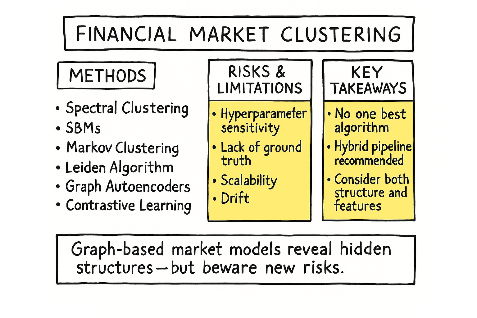
Introduction.
The network paradigm.
Model risks and limitations.
Spectral clustering.
Stochastic block models.
Markov clustering.
Leiden algorithm.
Graph autoencoders.
Contrastive learning.
Before you begin, remember that you have an index with the newsletter content organized by clicking on “Read full story” in this image.

Introduction
Look, here’s the thing—we’ve all been drinking the correlation Kool-Aid for decades, right? It’s elegant, sure. Clean math. Easy to explain to the PMs. But let’s get real: relying on a correlation matrix in today’s markets is like trying to sail a speedboat with an anchor chained to your hull. It’s not just simplistic—it’s dangerously misaligned with how the game actually works.
You think about it: correlations are backward-looking, linear, and static. Markets? They’re non-linear, regime-shifting, and chaotic . When volatility spikes, everything you thought was diversified suddenly moves in lockstep. Why? Because your pairwise analysis missed the latent feedback loops, the common risk factors blowing up across assets. You’re not measuring systemic risk—you’re just ignoring it until it bites you.
We lived this nightmare in 2018 during the volatility singularity. Not a Black Swan—everyone saw it coming. But our models? They were dead weight. Inverse-vol strategies blew up, futures cascaded into liquidation hell, and suddenly your low-correlation portfolio looked like a bunch of lemmings jumping off a cliff. Diversification? Gone. Hedging? Useless. Because the tools we used couldn’t see the dependencies hiding in plain sight.
So what’s the fix? You can’t just tweak the old models. You need to rip the playbook up and start over. There's much more to it than just matrices. There's much more to it than just matrices. Before we look at online clustering models in future articles, I want to take a moment to consider a different approach.
Model assets as nodes in a graph—dynamic, interconnected, with edges that evolve:
Use centrality measures to find the drivers.
Build minimum spanning trees to map contagion pathways.
Apply random matrix theory to filter noise from signal in eigenvalues.
The path forward required a complete abandonment of the flawed correlation matrix in favor of a graph-theoretic representation of the market. We shifted from viewing assets as solitary entities with simple pairwise handshakes to seeing them as nodes in a dynamic, living, and breathing system.
Take a look at this paper, it will serve as an index:

Okay, before we continue, I want to make one thing clear. These tools aren't for generating signals, but rather for contextualizing the market. That said, let's get started!
The network paradigm
A correlation matrix fails because it fundamentally atomizes the market. It presents a world of isolated relationships, ignoring the complex web of influence that truly governs financial dynamics. The relationship between Apple and Microsoft is not a simple, self-contained story. It is deeply modulated by their shared dependencies on the semiconductor industry (e.g., TSMC, NVDA), their competition in the consumer technology space, their collective sensitivity to macroeconomic policy, and the subtle shifts in sentiment flowing through the entire system. A graph, formally denoted as G=(V, E), provides a far richer and more honest framework.
Here, the assets are vertices (V), and their relationships—the edges (E)—can capture a universe of nuance.
The power of this paradigm lies in its expressive flexibility. Edge weights, wij, are no longer confined to the Pearson correlation coefficient. They can be engineered to represent more sophisticated concepts:
Mutual information: A measure from information theory that captures any statistical dependency, linear or non-linear, between two assets' return distributions.
Granger causality: A statistical test to determine if the past returns of one asset can be used to forecast the future returns of another, hinting at directional influence.
Shared factor exposure: The degree to which two assets are exposed to the same latent risk factors derived from models like PCA or deep autoencoders.
This leap from a flat matrix to a structured graph unlocks a new dimension of structural analysis. We can finally move beyond the myopic view of individual connections and begin to analyze the market's grand architecture. The questions we can now ask are vastly more insightful:
Centrality:
Centrality measures identify the most influential nodes in the network, the assets that are systemically important in ways a simple market cap weighting would miss.
Degree centrality: The number of direct connections a node has. An asset with high degree centrality is a local information hub. In trading terms, this might be a bellwether stock like JPMorgan in the financial sector, whose daily movements have a direct and immediate impact on a large number of other financial instruments.
Betweenness centrality: Measures how often a node lies on the shortest path between two other nodes. An asset with high betweenness centrality acts as a crucial bridge, connecting disparate clusters of the market. Think of a major logistics company like UPS; it may not be the largest company in any one sector, but it is fundamentally critical for connecting the manufacturing, retail, and consumer clusters. Its distress can signal a breakdown in the broader economic machine.
Eigenvector centrality: This is a more subtle measure of influence. A node has high eigenvector centrality if it is connected to other nodes that are themselves highly connected. This identifies assets that are central to the most important conversations in the market. Google is a prime example; it is not just highly connected, it is connected to other giants like Apple, Amazon, and Microsoft, making it a core component of the market's structure.
Community structure:
The core of the article is the search for communities—robust clusters of assets that behave as cohesive economic blocs. These are groups of stocks that are densely interconnected internally but only sparsely connected to the rest of the market. Identifying these functional groups, which often defy traditional sector classifications like GICS, is the first step toward building a truly diversified portfolio based on behavior, not labels.
Network typology:
Does the market exhibit small-world properties—where any asset is just a few steps away from any other—or scale-free properties?—where a few hub nodes have a vast number of connections, following a power law. Understanding these deep structural characteristics is critical for modeling how shocks are likely to propagate. A scale-free market is more resilient to random failures but terrifyingly vulnerable to targeted attacks on its central hubs.
The primary obstacle to adopting this paradigm was not technical, but cultural. It demanded that a team fluent in the comfortable world of linear algebra develop a new literacy in the abstract and sometimes counter-intuitive language of graph theory.

Model risks and limitations
To believe that the adoption of graph-theoretic models is a panacea is to swap one form of naivety for another. While our new map is undeniably more truthful than the old, it is also vastly more complex, and complexity is a fertile breeding ground for new and more subtle forms of risk. Acknowledging these perils is not a sign of weakness but the hallmark of a mature quantitative process. The most dangerous model is the one whose limitations are not understood.
Hyperparameters and model instability:
The elegant theories underpinning these models often conceal a messy reality: their performance is highly sensitive to the choice of hyperparameters. This is a crucial and challenging task. For the deep learning models—GAE, ARGA, MVGRL—we must specify learning rates, the dimensions of latent spaces, the number of GCN and fully-connected layers, and the number of training epochs. A slight change in the latent dimension from 32 to 64 can dramatically alter the resulting cluster topology.
This problem is not unique to deep learning. The Markov clustering algorithm's output is governed by the
inflationparameter; a value of 1.5 might yield a few large communities, while 2.5 could fracture the market into dozens of micro-clusters.The optimal set of hyperparameters for today's market data may be suboptimal tomorrow. This creates a risk of overfitting to a specific market regime, leading to models that are brittle and fail to generalize—a far more insidious problem than the straightforward failures of the correlation matrix.
Ground truth:
A fundamental epistemological risk lies in the fact that, in financial markets, there is no such thing as objective ground truth for clusters. The academic datasets used to benchmark these algorithms, come with predefined class labels. This allows for the calculation of clean evaluation metrics like Accuracy, Normalized Mutual Information, and Adjusted Rand Index.
Scalability:
While our experiments were on standard benchmarks, a financial graphs can contain millions of nodes—individual securities, options contracts, derivatives—and billions of edges.
The O(n³) complexity of a full eigendecomposition for Spectral Clustering makes it infeasible for a universe of more than a few thousand assets.
While GNNs are more scalable, training them on massive graphs is a significant computational and engineering feat. It requires specialized hardware and specific data pipelines for constructing and updating the graphs, and considerable expertise in distributed computing.
This computational burden is not just a one-time cost. For these models to be effective, they must be retrained frequently.
Drift:
Perhaps the greatest risk of all is that the market itself refuses to sit still. The graph structures we so carefully identify are transient. The communities that define the market today can and will dissolve tomorrow. A merger, a technological breakthrough, a geopolitical event, or a simple shift in investor sentiment can instantly rewire the network.
All of these models are trained on historical data, and thus they carry an implicit assumption of stationarity. They are excellent at finding the structure in the data they have seen, but they are not clairvoyant. The phenomenon of concept drift—where the statistical properties of the target variable change over time—is the primary antagonist in all of financial modeling.
Spectral clustering
Once the market is mapped as a graph, the immediate imperative is to partition it into its constituent communities. We need to find those dense clusters of assets that move together, breathe together, and, in times of crisis, fall together. Spectral clustering is a way to do this task. Unlike distance-based algorithms like k-means, which flounder in the high-dimensional, non-Euclidean space of financial assets, Spectral clustering operates on the very soul of the graph: its connectivity structure.
The magic of the method comes from the Graph Laplacian, a matrix that is central to graph theory. It is formally defined as L=D−A, where A is the graph's weighted adjacency matrix and D is the diagonal degree matrix containing the sum of weights for each node. The Laplacian is a discrete analogue of the Laplace operator from vector calculus and it encodes information about the graph's structure. Its spectrum—the set of its eigenvalues and their corresponding eigenvectors—reveals the most natural cuts in the network fabric.
The key insights are as follows:
The smallest eigenvalue of a Laplacian is always 0.
The number of zero eigenvalues is equal to the number of connected components in the graph. A market graph should ideally be one single component.
The eigenvector corresponding to the second-smallest eigenvalue, lambda2 often called the Fiedler vector, holds the key to the graph's most fundamental partition. The signs of its elements (+ or -) naturally bisect the graph into two well-separated communities.
To find k clusters, we don't just use the Fiedler vector. We compute the first k eigenvectors corresponding to the k smallest non-zero eigenvalues. We then stack these eigenvectors column-wise to form a new matrix U∈Rnxk, where n is the number of assets. Each row of this matrix is a new, low-dimensional coordinate for an asset—a spectral embedding.
In this transformed space, the messy, high-dimensional clusters become trivially separable, and we can deploy a simple algorithm like k-means to finish the job. This technique effectively uncovers functional asset groupings that transcend traditional, and often arbitrary, GICS sector labels.
The search for these eigenvectors can be framed as an optimization problem via the Min-Max Courant-Fisher theorem. The second-smallest eigenvalue lambda2, for instance, is the solution to:
where d is the eigenvector for lambda1=0 (a vector of ones). The term xTLx has a beautiful interpretation, as revealed by the Rayleigh theorem:
Minimizing this expression means assigning values xi to each node such that the squared differences across connected nodes are small. Intuitively, this forces nodes within a dense cluster to have very similar x values, while nodes in different clusters will have dissimilar values, creating a cut.
Here is the snippet for the workflow.
import numpy as np
from sklearn.cluster import KMeans
from scipy.sparse import csgraph
import matplotlib.pyplot as plt
import seaborn as sns

def spectral_clustering_implementation(returns_matrix, num_clusters=5, threshold=0.5):
    """
    Performs Spectral Clustering on an asset returns matrix. This method leverages the
    eigenvectors of the graph Laplacian to find meaningful clusters in the data.

    Args:
        returns_matrix (np.ndarray): A matrix of asset returns where rows are assets
                                      and columns are time steps (e.g., daily returns).
        num_clusters (int): The desired number of clusters to partition the assets into.
        threshold (float): A value from 0 to 1 to prune weak correlations, creating a
                           sparser, more meaningful graph. Edges with weights below this
                           are set to zero.

    Returns:
        tuple: A tuple containing:
               - np.ndarray: An array of cluster labels assigning each asset to a cluster.
               - np.ndarray: The low-dimensional spectral embedding of the assets.
               - np.ndarray: The eigenvalues of the Laplacian.
    """
    print("1. Calculating the asset-asset correlation matrix from returns...")
    # np.corrcoef calculates the Pearson correlation coefficient between rows.
    # The result is a symmetric matrix where C[i, j] is the correlation between asset i and j.
    corr_matrix = np.corrcoef(returns_matrix)

    # We use the absolute value of the correlation as a measure of affinity (similarity).
    # A strong negative correlation is just as significant a relationship as a strong positive one.
    affinity_matrix = np.abs(corr_matrix)
    # Prune weak connections to reduce noise and focus on strong relationships.
    affinity_matrix[affinity_matrix < threshold] = 0
    # The diagonal should be 1, representing an asset's perfect correlation with itself,
    # but for graph purposes, self-loops are often handled separately or set to 0.
    np.fill_diagonal(affinity_matrix, 0)

    print(f"2. Affinity matrix created with shape: {affinity_matrix.shape}")

    print("3. Computing the unnormalized Graph Laplacian (L = D - A)...")
    # The csgraph.laplacian function from scipy is numerically stable and efficient.
    # 'normed=False' specifies the unnormalized Laplacian.
    laplacian_matrix = csgraph.laplacian(affinity_matrix, normed=False)

    print("4. Performing eigendecomposition to find the spectrum of the Laplacian...")
    # We need the eigenvectors corresponding to the smallest eigenvalues.
    # np.linalg.eigh is optimized for symmetric matrices like the Laplacian.
    eigenvalues, eigenvectors = np.linalg.eigh(laplacian_matrix)

    print(f"5. Creating spectral embedding with the first {num_clusters} non-trivial eigenvectors...")
    # The first eigenvector (at index 0) corresponds to the smallest eigenvalue (ideally 0 for a
    # connected graph) and is a constant vector, providing no clustering information.
    # We take the next 'num_clusters' eigenvectors to form our new feature space.
    spectral_embedding = eigenvectors[:, 1:num_clusters+1]

    print("6. Running K-Means on the low-dimensional spectral embedding...")
    # K-Means is highly effective in this new space, as the clusters are well-separated.
    kmeans = KMeans(n_clusters=num_clusters, random_state=42, n_init='auto')
    clusters = kmeans.fit_predict(spectral_embedding)

    print("7. Spectral Clustering complete.")
    return clusters, spectral_embedding, eigenvalues

# Main
if __name__ == "__main__":
  # Generate a mock returns matrix for 50 assets over 252 days (1 trading year)
  np.random.seed(5)
  num_assets = 50
  num_days = 252
  mock_returns = np.random.randn(num_assets, num_days)

  # Add some latent structure: make groups of assets correlated to simulate sectors.
  mock_returns[0:10, :] += np.random.randn(1, num_days) * 0.5  # Cluster 1
  mock_returns[10:25, :] += np.random.randn(1, num_days) * 0.5 # Cluster 2
  mock_returns[25:35, :] += np.random.randn(1, num_days) * 0.5 # Cluster 3
  # Cluster 4 is the remaining uncorrelated assets

  # Perform spectral clustering
  asset_clusters, embedding, evals = spectral_clustering_implementation(mock_returns, num_clusters=4, threshold=0.1)

  print(f"\nCluster assignments for {num_assets} assets:")
  print(asset_clusters)
We have generated two different plots:
Eigengap plot: This visualizes the first few eigenvalues of the Laplacian in increasing order. A common heuristic for determining the optimal number of clusters, k, is to look for a large gap between consecutive eigenvalues. The value of k is chosen to be the number of eigenvalues before this gap. This gap signifies that any further partitions would require cutting through a much denser part of the graph, making them less natural.
Spectral embedding plot: This is a scatter plot of the assets in their new coordinate system, defined by the first two meaningful eigenvectors—the Fiedler vector and the 3rd eigenvector. In this new space, the clusters which were tangled and inseparable in the original high-dimensional space now appear as distinct, well-separated clouds of points.
Stochastic block models
Spectral Clustering provides a deterministic snapshot of the market's structure. However, as you already know, the market is anything but deterministic. To capture this inherent randomness and to model the market's structure we turn to Stochastic block models. SBMs take graph partitioning into the realm of statistical inference. Instead of just finding a single best partition, an SBM attempts to learn a probabilistic model of the market's latent community structure itself.
The core assumption of an SBM is that each asset i belongs to one of K hidden communities, represented by a membership vector z. The probability of an edge existing between two assets i and j then depends only on the communities to which they belong, zi and zj. The goal of the inference process is to find the community assignments z and the K × K inter-community probability matrix B that maximize the likelihood of observing the actual market graph A:
where theta=(B, z) are the model parameters. This is an interesting shift. We are no longer just describing the network; we are building a generative model that could, in theory, produce other market graphs with the same underlying community.
This model-based approach allows for:
Statistical inference: We can place confidence intervals on our cluster assignments and the inter-block connection probabilities.
Model selection: Principled methods like Bayesian Information Criterion or cross-validation can be used to determine the optimal number of latent communities, K.
The matrix B provides a concise summary of the entire market's mesoscale structure. We can see which communities are closely allied (high Brs), which are isolated, and which act as bridges.
For financial markets, however, the standard SBM has a crippling flaw. It operates under the assumption of stochastic equivalence, meaning all nodes within the same block are statistically interchangeable in their connection patterns. This is patently false in finance. A community like big tech contains both behemoth hubs like Amazon and smaller, more peripheral players. They are not equivalent.
The essential upgrade is the Degree-Corrected SBM. The DC-SBM introduces an additional parameter thetai for each node, which controls its expected degree. This allows for massive heterogeneity of degrees within a single community. A hub and a peripheral stock can now coexist peacefully in the same cluster, distinguished by their theta values but united by their shared pattern of connections to other communities. This is a far more realistic model of market structure.
Inference for SBMs is typically performed using iterative algorithms like the Expectation-Maximization algorithm or variational inference methods.
Let’s code it:
# !pip install scikit-network

import numpy as np
import matplotlib.pyplot as plt

def compute_likelihood(A, g, K):
    """
    Compute the (degree-corrected) SBM log-likelihood (up to a constant)
    for adjacency A and assignments g∈{0,…,K-1}.
    """
    N = A.shape[0]
    # Node degrees
    k = A.sum(axis=1)
    # Sum of degrees per block
    kappa = np.array([k[g == r].sum() for r in range(K)])
    # Edge counts between blocks (double-counts for r≠s; diagonal zero-diagonal)
    M = np.zeros((K, K))
    for r in range(K):
        for s in range(K):
            M[r, s] = A[np.ix_(g == r, g == s)].sum()

    L = 0.0
    for r in range(K):
        for s in range(r, K):
            m_rs = M[r, s]
            if m_rs <= 0:
                continue
            if r == s:
                # intra-block term (M_rr is double-counted edges)
                L += m_rs * np.log(m_rs / (kappa[r] * kappa[r]))
            else:
                # inter-block term
                L += 2 * m_rs * np.log(m_rs / (kappa[r] * kappa[s]))
    return L

def degree_corrected_sbm(A, K, max_iter=100, random_state=42, verbose=False):
    """
    Greedy maximize DC-SBM likelihood by re-assigning one node at a time.
    """
    N = A.shape[0]
    rng = np.random.RandomState(random_state)
    # random initial assignment
    g = rng.randint(K, size=N)
    L = compute_likelihood(A, g, K)
    if verbose:
        print(f"Initial likelihood: {L:.4f}")

    for it in range(max_iter):
        moved = False
        for i in range(N):
            best_r, best_L = g[i], L
            for r in range(K):
                if r == g[i]:
                    continue
                g_tmp = g.copy()
                g_tmp[i] = r
                L_tmp = compute_likelihood(A, g_tmp, K)
                if L_tmp > best_L:
                    best_r, best_L = r, L_tmp
            if best_r != g[i]:
                if verbose:
                    print(f" Iter {it}, move node {i} → {best_r}, ΔL={(best_L - L):.4f}")
                g[i], L = best_r, best_L
                moved = True
        if not moved:
            if verbose:
                print(f"Converged after {it} iterations.")
            break
    return g

def sbm_clustering_implementation(returns_matrix, num_clusters=5, threshold=0.5,
                                  max_iter=100, random_state=42, verbose=False):
    """
    Performs degree‐corrected SBM clustering on asset returns.

    Args:
      returns_matrix (np.ndarray): assets × time returns.
      num_clusters (int): number of communities.
      threshold (float): binarize |
        corr| > threshold → edge.
      max_iter (int): max passes for greedy optimization.
      random_state (int): seed for reproducibility.
      verbose (bool): print progress.

    Returns:
      clusters (np.ndarray): cluster label in {0..num_clusters-1} for each asset.
      adjacency_matrix (np.ndarray): the binarized graph.
    """
    # 1. compute asset–asset correlations
    corr = np.corrcoef(returns_matrix)
    # 2. threshold to get an unweighted graph
    A = (np.abs(corr) > threshold).astype(int)
    np.fill_diagonal(A, 0)

    if verbose:
        print("Adjacency matrix built — running DC-SBM...")

    clusters = degree_corrected_sbm(
        A, num_clusters,
        max_iter=max_iter,
        random_state=random_state,
        verbose=verbose
    )
    if verbose:
        print("Clustering complete.")
    return clusters, A

# Main
if __name__ == "__main__":
    np.random.seed(42)
    num_assets = 50
    # simulate 1 year of daily returns
    mock_returns = np.random.randn(num_assets, 252)
    # inject two correlated groups
    mock_returns[ 0:10, :] += np.random.randn(1, 252) * 0.5
    mock_returns[10:25, :] += np.random.randn(1, 252) * 0.5

    sbm_clusters, sbm_adj = sbm_clustering_implementation(
        mock_returns,
        num_clusters=4,
        threshold=0.2,
        max_iter=50,
        verbose=True
    )
    print("\nCluster assignments:", sbm_clusters)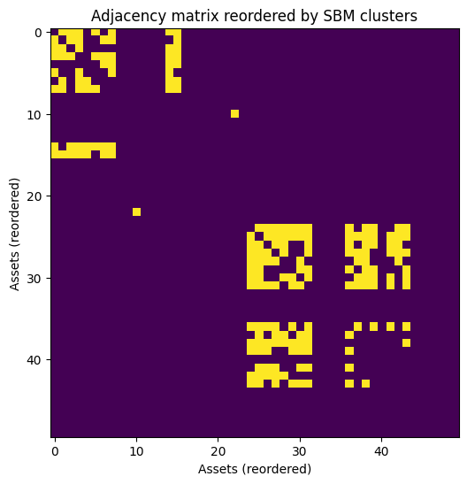
The code generates a heatmap of the adjacency matrix after its rows and columns have been reordered according to the cluster assignments found by the SBM. Instead of a noisy, seemingly random pattern of connections, the reordered matrix will reveal a clear block structure. Dense, bright squares appear along the diagonal, representing the high intra-cluster connectivity. The off-diagonal regions are sparse and dark, representing the low inter-cluster connectivity.

Markov clustering
While SBMs reveal a static, probabilistic blueprint of the market, they don't explicitly model the dynamics that occur on the network. For a quant, the most important dynamic is the flow of capital and information.
The Markov clustering algorithm is an intuitive method designed to discover community structure by simulating just such a flow process on the market graph. It's a process that mimics how a random walker, if left to wander the graph, would naturally get stuck in densely connected regions.
The algorithm is a dance between two simple yet powerful steps, iterated until the network fractures into its natural basins of attraction:
Expansion: This step simulates the spread of flow across the network. Mathematically, it involves taking the graph's transition matrix P—where Pij is the probability of moving from node i to node j in one step—and raising it to a power, e. The new matrix Pe represents the probabilities of reaching any node from any other node in e steps. This has the effect of thickening connections within existing clusters. If two nodes are in the same dense community, there are many paths between them, and expansion makes these paths more prominent, increasing the probability of flow staying within the community.
Expansion of power e:
\(P^{(e)} \;=\; P^e\)which spreads flow along paths of length e.
Inflation: This is the crucial, non-linear step that enforces partitioning. We take the expanded matrix and apply an element-wise power, r—the inflation parameter—and then re-normalize each column to ensure it remains a valid probability distribution. This is a classic rich-get-richer scheme. High-probability transitions—strong connections within clusters—become quadratically or cubically stronger, while low-probability transitions—weak links between clusters—are suppressed and wither away towards zero. Inflation sharpens the boundaries between communities.
Inflation with parameter r: apply the entrywise power r and then re-normalize each column to sum to 1:
\(\bigl[\Gamma_r(P^{(e)})\bigr]_{ij} \;=\; \frac{\bigl(P^{(e)}_{ij}\bigr)^r} {\displaystyle\sum_{k=1}^n \bigl(P^{(e)}_{kj}\bigr)^r}\)Putting these together, the MCL operator Me,r on P is:
\(P \;\mapsto\; \mathcal{M}_{e,r}(P) \;=\; \Gamma_{r}\bigl(P^{e}\bigr).\)
By alternating between expansion—exploring—and inflation—exploiting—the flow matrix converges to a steady state. This final matrix is sparse, composed of disconnected blocks of non-zero probabilities. The flow becomes trapped within these regions, which are precisely the graph's most stable communities.
For trading, these are the natural homes for capital, the asset groups that are most robust to the simulated ebbs and flows of market information. The inflation parameter, r, acts as a knob for controlling the granularity of the clusters; higher values of r lead to more numerous, smaller, and tighter clusters.
Let’s implement it:
# !pip install markov_clustering

import numpy as np
import markov_clustering as mc
import networkx as nx

def mcl_clustering_implementation(returns_matrix, inflation=1.5, threshold=0.5):
    """
    Performs Markov Clustering (MCL) on asset returns by simulating flow.

    Args:
        returns_matrix (np.ndarray): Matrix of asset returns (assets x time).
        inflation (float): The key MCL parameter. Higher values (>2.0) lead to more
                           granular (smaller, tighter) clusters. Values between 1.2-2.0
                           are common starting points.
        threshold (float): Correlation threshold for graph construction.

    Returns:
        tuple: A tuple containing:
               - list: A list of tuples, where each tuple contains the indices of assets in a cluster.
               - np.ndarray: A mapping from asset index to a numerical cluster ID.
               - networkx.Graph: The graph object used for visualization.
    """
    print("1. Calculating correlation and building affinity matrix for MCL...")
    corr_matrix = np.corrcoef(returns_matrix)
    # MCL operates on a weighted adjacency matrix, representing flow probabilities.
    affinity_matrix = np.abs(corr_matrix)
    affinity_matrix[affinity_matrix < threshold] = 0
    # MCL requires non-negative weights. It internally adds self-loops and normalizes
    # to create a stochastic transition matrix.
    np.fill_diagonal(affinity_matrix, 0)

    print(f"2. Running MCL with inflation parameter: {inflation}...")
    # The mc.run_mcl function performs the expansion and inflation steps until convergence.
    result = mc.run_mcl(affinity_matrix, inflation=inflation)

    # The result is the converged matrix. mc.get_clusters extracts the clusters by
    # finding the connected components (attractors) in this final graph.
    clusters = mc.get_clusters(result)

    print("3. MCL clustering complete.")

    # For convenience and visualization, create a mapping from each asset's index to its cluster ID.
    num_assets = returns_matrix.shape[0]
    cluster_map = np.zeros(num_assets, dtype=int)
    for cluster_id, cluster_nodes in enumerate(clusters):
        for node_index in cluster_nodes:
            cluster_map[node_index] = cluster_id

    # Create a NetworkX graph for visualization
    graph = nx.from_numpy_array(affinity_matrix)

    return clusters, cluster_map, graph

# Main
if __name__ == "__main__":
np.random.seed(42)
num_assets = 50
mock_returns = np.random.randn(num_assets, 252)
mock_returns[0:10, :] += np.random.randn(1, 252) * 0.5
mock_returns[10:25, :] += np.random.randn(1, 252) * 0.5

# Perform MCL clustering
  mcl_clusters, mcl_map, mcl_graph = mcl_clustering_implementation(mock_returns, inflation=1.8, threshold=0.2)
  print(f"\nMCL found {len(mcl_clusters)} clusters.")
  print("Cluster mapping for each asset:")
  print(mcl_map)
The code produces a network graph visualization where nodes or assets are positioned based on their connectivity using a force-directed layout. Each node is then colored according to the cluster it was assigned to by the MCL algorithm.
The Leiden algorithm
As our asset universe expanded from hundreds to thousands of instruments, a new a obstacle emerged: computational scale. The Spectral clustering, with its O(n³) complexity for eigendecomposition, became prohibitively slow. We needed an algorithm that is not only accurate but also fast. This led us to the family of modularity optimization algorithms.
Modularity, denoted by Q, is a quality metric that quantifies how good a particular partition of a graph is. It measures the fraction of edges that fall within the given clusters minus the expected fraction if edges were distributed randomly, preserving node degrees. The formula is:
where m is the total number of edges, Aij is the adjacency matrix, ki is the degree of node i, ci is the community of node i, and delta is the Kronecker delta (1 if ci=cj, 0 otherwise). A high modularity score indicates a partition with dense internal connections and sparse external ones—precisely what we are looking for.
The popular Louvain method is a greedy algorithm designed to rapidly find partitions with high modularity. It's incredibly fast, but our research uncovered a critical, subtle flaw:
It can identify dendritic communities that, while having a high modularity score, are internally fractured and held together by just a few weak links. For building a trading portfolio, relying on such a fragile community is an unacceptable risk.
The Leiden algorithm is the direct successor to Louvain, engineered specifically to solve this problem. It follows the same fast, hierarchical approach but introduces a clever refinement phase. After greedily moving nodes, it attempts to split the newly formed communities. This guarantees that all reported communities are not just abstract groups but are themselves well-connected subgraphs.
For finance, this guarantee of internal cohesion is key. It ensures that the communities we identify are truly robust and can form the basis of a diversified portfolio that won't shatter under stress.
The algorithm iterates through three phases until no improvements can be made:
Local node movement: Greedily move individual nodes to neighboring communities to achieve the largest local increase in modularity.
Refinement: Attempt to break apart the communities formed in the first phase to find better, more cohesive sub-partitions.
Aggregation: Create a new, smaller network where the nodes are the communities found in the previous step. Repeat the process on this aggregated network.
Let’s code it: