

[WITH CODE] Model: FURIA algorithm
Build rules that breathe with the market, not break under pressure

Table of contents:
Introduction.
Assessing limitations.
Embracing fuzzy logic as a strategic catalyst.
Theoretical framework of fuzzy rule induction.
Purity and certainty in fuzzy rule evaluation.
The FURIA algorithm.
Before you begin, remember that you have an index with the newsletter content organized by clicking on “Read full story” in this image.

Introduction
Let’s be real—markets are messy, volatile beasts. For years, algo strategies have leaned on these crisp, binary rules: If X crosses threshold Y, execute Z. But anyone who’s spent time on a trading floor knows markets don’t play by tidy rules. Take a classic momentum signal—say, a ‘buy’ trigger when price breaches a moving average. The second that threshold gets crossed, you’re supposed to act. But here’s the rub: markets don’t flip a switch. That ‘buy’ signal might fire while the broader context—liquidity, volatility, order flow—is still in this murky transition. It’s like slapping a ‘storm warning’ on a radar blip that’s still just a ripple.
So now you’re stuck with this quant dilemma: How do you teach machines to navigate ambiguity when their entire framework is built on yes/no logic? Standing there, staring at screens drowning in noise, it hits you—forcing binary decisions on markets is like trying to track a hurricane with a light switch. You’re either ‘on’ or ‘off,’ while the storm rages in gradients.

Assessing limitations
To build a robust trading system, we must confront several risks imposed by conventional rule-based systems:
Loss of nuance: Traditional classifiers that enforce hard decision boundaries provide no margin for error, often leading to frequent rebalancing and overtrading as market conditions oscillate around a fixed threshold.
Systematic biases: Ordered rule lists, common in methods like RIPPER, tend to privilege one class—often the default or majority class. In trading, this bias can result in a persistent overexposure to certain market conditions.
Inflexible adaptation: The inability to deal with uncovered instances—i.e., those market conditions that do not neatly satisfy any crisp rule—forces traders to rely on default actions that may be suboptimal.
Inadequate risk management: Abrupt transitions can lead to higher transaction costs, slippage, and adverse selection. All these factors compound to worsen the overall trading performance.
These risks are paralleled in any system that fails to model uncertainty. Markets do not respond in binary fashion; they rather exhibit a continuum of responses based on partially observable factors, leading to the conclusion that a more nuanced approach is needed.
If you're curious, don't miss this article in which I develop the RIDRA algorithm:

Embracing fuzzy logic as a strategic catalyst
The pivotal moment comes with the realization that fuzzy logic offers the perfect antidote to the rigidity of crisp rule-based models. Fuzzy logic introduces the concept of graded membership, in which data points can belong to a set to a certain degree rather than in an absolute manner.
Imagine a trader no longer making decisions solely on whether a price is above or below a specific value, but rather, assessing the degree to which the price aligns with a bullish or bearish condition. This is analogous to a spectrum rather than a binary state. By replacing sharp decision boundaries with soft fuzzy intervals, we can simulate the gradual transitions common in the market data.
The Fuzzy Unordered Rule Induction Algorithm (FURIA) is built on this very philosophy. It modifies the state-of-the-art RIPPER algorithm by:
Learning fuzzy rules: FURIA replaces conventional crisp rules with fuzzy rules that have gradual membership functions.
Unordered rule sets: Instead of imposing an order that may bias the model, FURIA learns rules for each class independently in a one-vs.-rest manner.
Rule stretching: To manage uncovered examples—market states that lie in-between preset conditions—FURIA utilizes a rule stretching mechanism that generalizes rules in a local, data-driven way.

This breakthrough is the catalyst for a new class of algorithmic trading systems—one that can adapt to the fluid, ambiguous nature of financial markets.
If you want to check it out in more depth, check out this paper:

Theoretical framework of fuzzy rule induction
Before diving into implementation details, we must first establish a firm mathematical foundation. Fuzzy logic extends classical set theory by allowing partial membership. Instead of an element belonging fully to a set or not at all, fuzzy sets enable degrees of membership. A common representation is the trapezoidal membership function. Consider a financial indicator x—for instance, a normalized momentum score. A fuzzy set IF representing “bullish momentum” may be defined by a trapezoidal function with four parameters:
The corresponding membership function is given by:
Here, ϕc,L and ϕc,U define the core—complete membership region—and ϕs,L and ϕc,U define the support—the transition zones. In trading, this gradual transition is analogous to assessing the degree of bullishness of a market condition rather than a binary yes/no.
Furthermore, for a fuzzy rule composed of k conditions—for different market indicators—the overall degree of coverage of an instance x—a vector of market data—is given by the product of the individual memberships:
This multiplicative aggregation reflects the joint likelihood that the market condition x is consistent with a given rule. Higher values indicate a stronger match.
Purity and certainty in fuzzy rule evaluation
To fine-tune fuzzy rules, FURIA uses the concept of purity. For a given rule, let:
p be the weighted sum of positive—target—instances,
n be the weighted sum of negative instances, with weights given by the fuzzy membership of each instance. The purity is then expressed as:
This metric is later used to choose the best candidate support boundaries during fuzzification.
The certainty factor for a rule—a value that adjusts the contribution of the rule in classification—is computed using a modified Laplace estimate:
where p and n are defined as before. This factor weighs each rule’s impact and is particularly crucial when multiple fuzzy rules are aggregated for decision making.
The FURIA algorithm
The original FURIA algorithm re-engineers the classical RIPPER algorithm with three significant modifications:
Fuzzy transformation: Traditional crisp rules—with hard decision boundaries—are converted into fuzzy rules by replacing strict intervals with fuzzy intervals—as described above. This makes rules softer and more adaptable to gradual changes in market data.
Unordered rule sets: Instead of creating an ordered rule list—which might bias the system toward a default class—FURIA learns an unordered set of rules using a one-vs.-rest approach. In algorithmic trading, this equal treatment ensures that all market states are evaluated fairly, without undue bias toward regular conditions.
Rule stretching: To handle instances that are not covered by any rule, FURIA employs a local strategy called rule stretching. In this process, a rule is generalized—by dropping one or more conditions—until it covers the query instance. Unlike a default rule, rule stretching leverages the local structure of the market data to adjust decisions dynamically.
Together, these modifications yield a robust classification system that can effectively map fuzzy market indicators into actionable trading signals. So the pseudo-code looks like this:
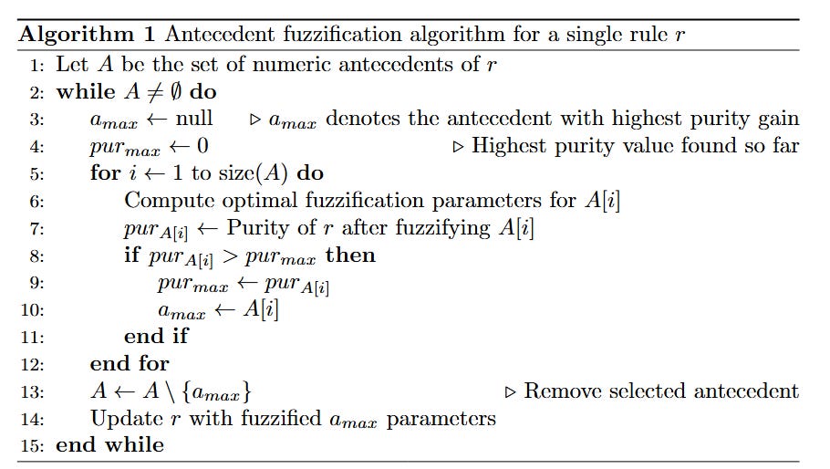
Now that we have a clear understanding, it’s time to code it!
The following function computes the trapezoidal membership, which is central to our fuzzy rule evaluation. In algorithmic trading, this may be used to assess the degree to which an indicator—e.g., RSI or moving average deviation, although I prefer to use another type of data for this type of algos—belongs to a bullish or bearish set.
import numpy as np
import matplotlib.pyplot as plt
def trapezoidal_membership(x, a, b, c, d):
"""
Compute the trapezoidal membership function for value(s) x.
a: left support
b: left core
c: right core
d: right support.
"""
x = np.array(x)
mu = np.zeros_like(x, dtype=float)
# Rising edge
rising = (x > a) & (x < b)
if (b - a) != 0:
mu[rising] = (x[rising] - a) / (b - a)
else:
mu[rising] = 1.0
# Core region
core = (x >= b) & (x <= c)
mu[core] = 1.0
# Falling edge
falling = (x > c) & (x < d)
if (d - c) != 0:
mu[falling] = (d - x[falling]) / (d - c)
else:
mu[falling] = 1.0
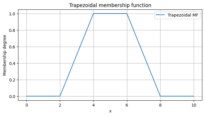
return muImagine plotting μ(x) on the y-axis against x on the x-axis. With parameters a=2, b=4, c=6, and d=8, the function rises from 0 to 1 between 2 and 4, remains at 1 until 6, and then falls off to 0 at 8. In trading, such a smooth curve allows for measuring the degree of bullishness as market indicators vary gradually. Like this:
On the other hand, we define a FuzzyCondition class that encapsulates conditions such as indicator ≤ threshold or indicator > threshold. Each condition has a core—where the rule holds completely—and a support—representing transition.
class FuzzyCondition:
    """
    Represents a fuzzy condition derived from a crisp rule.
    For "feature <= threshold", the crisp threshold is the core bound, and support is set with an offset delta.
    """
    def __init__(self, feature_idx, op, threshold, delta=1.0):
        self.feature_idx = feature_idx
        self.op = op  # can be "<=" or ">"
        self.threshold = threshold
        if op == '<=':
            self.phi_c = threshold       # Core: all values ≤ threshold are fully in the set.
            self.phi_s = threshold + delta  # Support: values above threshold until this point have decreasing membership.
        elif op == '>':
            self.phi_c = threshold       # Core: all values > threshold.
            self.phi_s = threshold - delta  # Support: values below threshold until this point.
        else:
            raise ValueError("Operator must be '<=' or '>'")

    def membership(self, x_value):
        """
        Compute the fuzzy membership of x_value for this condition.
        """
        if self.op == '<=':
            if x_value <= self.phi_c:
                return 1.0
            elif x_value >= self.phi_s:
                return 0.0
            else:
                return (self.phi_s - x_value) / (self.phi_s - self.phi_c)
        elif self.op == '>':
            if x_value >= self.phi_c:
                return 1.0
            elif x_value <= self.phi_s:
                return 0.0
            else:
                return (x_value - self.phi_s) / (self.phi_c - self.phi_s)

    def fuzzify(self, X, y, pos_label):
        """
        Optimize the support boundary using training examples relevant to the condition.
        """
        feature_values = X[:, self.feature_idx]
        if self.op == '<=':
            candidates = feature_values[feature_values > self.threshold]
            if len(candidates) > 0:
                self.phi_s = np.min(candidates)
        elif self.op == '>':
            candidates = feature_values[feature_values < self.threshold]
            if len(candidates) > 0:
                self.phi_s = np.max(candidates)
A fuzzy rule is then built as a conjunction of multiple fuzzy conditions. In financial terms, a rule might combine several market indicators—e.g., moving average, momentum index or any other—into a composite trading signal.