[WITH CODE] Model: RIPPER rule-based algorithm

Extracting rules or inviting disaster? How decoding math can save your portfolio from market mayhem

---

Table of contents:

1. Introduction.

2. Foundations of Rule extraction.

   1. Boolean logic and Set theory → The building blocks.

   2. Probability and information theory → Measuring uncertainty.

   3. Optimization → Balancing simplicity and accuracy.

3. The RIPPER Algorithm.

   1. Implementing RIPPER.

   2. Extracting and displaying rules.

4. Final considerations.

---

Introduction

Let’s be real, in quant finance, everyone’s chasing that tiny edge—the kind that turns a “meh” model into a money-making machine. But here’s the thing: you can’t just throw data into a neural net, cross your fingers, and call it innovation. If you want to build rule extraction models that actually work—models that explain why they work—you need to get cozy with the math under the hood. Seriously, it’s not optional.

Rule extraction isn’t magic but it’s an option. It’s a blend of linear algebra, optimization, and probability theory wearing a fancy hat. Skip the fundamentals, and you’ll end up with a model that’s about as reliable as a weather forecast from a Magic 8-Ball. Sure, it might spit out rules that look good on paper, but when markets flip—and they always do—that thing will crumble faster than you can say overfitting. Worse, you’ll be stuck trying to explain its logic to a room full of skeptical risk managers.

Here’s the kicker: the quants who win long-term aren’t the ones glued to TensorFlow tutorials. They’re the ones who can rewrite the tutorials. They see matrices and manifolds not as homework problems, but as LEGO bricks for building smarter, faster, more transparent systems. Because when you speak math fluently, you don’t just iterate—you invent.

So yeah, you could treat rule extraction like a black box. Or you could crack it open, tweak its guts, and build something nobody’s seen before. Your call—but I know where the alpha’s hiding.

Foundations of Rule extraction

To understand how rule extraction works, we must first delve into the elegant mathematics that underpin these models.

Boolean logic and Set theory → The building blocks

The journey begins with the very language of rules—logic. At its simplest, a rule is an “if–then” statement. For example:

IF (Condition A AND Condition B) OR Condition C THEN Buy

Each condition, such as “SMA20 > SMA50,” is a Boolean expression that evaluates as either true or false. Boolean logic rests on three fundamental operations:

• Conjunction—AND, ∧: True only if both conditions are true.

• Disjunction—OR, ∨: True if at least one condition is true.

• Negation—NOT, ¬: Flips the truth value.

These operations obey laws—such as De Morgan’s laws—that help simplify and manipulate complex expressions. Think of Boolean logic as the digital alphabet that allows us to construct the sentences or rules which guide our decision-making processes.

Complementing Boolean logic is set theory. Envision your entire dataset as a universal set U. Each condition in a rule selects a subset of U. For instance, let:

• A be the set of instances where “Volume > 1000.”

• B be the set of instances where “Price > SMA.”

The rule “IF Volume > 1000 AND Price > SMA THEN Buy” is then represented by the intersection A∩B. Set theory not only provides visual intuition but also forms the basis for understanding rule coverage and the overlap between different conditions.

Probability and information theory → Measuring uncertainty

Having established the structural language of rules, we now turn to probability and information theory—the tools that measure how “good” a rule is.

1. Entropy quantification:

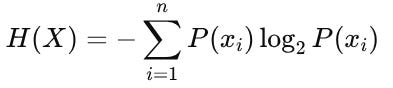
   Entropy is a metric that quantifies uncertainty or disorder within a dataset. In a scenario where all examples belong to a single class—say, “Buy”—entropy is zero because there is no uncertainty. Conversely, a perfectly mixed dataset exhibits high entropy. Mathematically, for a discrete random variable X with outcomes {x₁,x₂,…,x_n} and probabilities P(x_i):

   

   When we apply a rule, we aim to reduce this uncertainty—effectively “purer” subsets make for better predictions.

2. Information gain:

   Building on entropy, information gain measures the reduction in uncertainty when a dataset is partitioned by a condition. If a dataset D is divided into subsets D₁,D₂,…,D_k​ by a condition X, the information gain is defined as:

   

   A condition that offers high information gain is akin to finding a key that neatly organizes your data, making the subsequent decision-making process much clearer.

3. Conditional probability and rule confidence:

   Another layer of evaluation is provided by Bayesian probability. For a rule such as “IF condition THEN action,” the confidence is given by:

   

   This probability reflects how reliably the rule predicts the desired outcome when its conditions are met, ensuring that the rules we derive are not only logically sound but also statistically robust.

Optimization → Balancing simplicity and accuracy

Even with strong logical and probabilistic foundations, rules can become overly complex. Optimization techniques help us strike the right balance by minimizing errors while keeping rules as simple as possible.

1. Objective functions and regularization:

   To formalize this balance, we define an objective function that penalizes both misclassification error and complexity. One common formulation is:

   

   Where:

   • E(R) is the error rate of the rule set.

   • C(R) is a measure of its complexity—for example, the number of conditions.

   • λ is a regularization parameter that controls the trade-off.

   This approach is analogous to finding a recipe that is both delicious and straightforward—too many ingredients may overwhelm the dish, just as too many conditions can obscure the rule.

2. Greedy search and pruning:

   Since the space of all possible rules is enormous, greedy search algorithms help by incrementally adding the condition that offers the most improvement. However, to avoid overfitting—like trimming excess decoration off a well-crafted cake—we use pruning techniques to remove redundant conditions, thereby simplifying the rule while preserving its performance.

When Boolean logic and set theory meet probability and optimization, we obtain rule extraction models that are not only powerful but also interpretable. These premises transform raw, noisy data into clear if–then rules, revealing the underlying decision process in a manner that is both rigorous and accessible.

Let’s see a classic algorithm: RIPPER. It exemplifies this synthesis by growing rules and pruning them immediately, ensuring that each rule is statistically valid and elegantly simple.

The RIPPER Algorithm

With our mathematical foundation laid, we now turn to RIPPER (Repeated Incremental Pruning to Produce Error Reduction)—a rule induction algorithm that builds rule sets step by step. RIPPER works through the following stages:

1. Rule growing: Beginning with an empty rule, conditions are added one at a time—often using a measure like FOIL gain—until the rule performs adequately.

2. Rule pruning: Once a rule is grown, it is immediately pruned by removing conditions that do not significantly improve performance. This is guided by a split of the training data into a growing set and a pruning set.

3. Rule set construction: The process is repeated—each new rule is added to the rule set, and examples covered by that rule are removed from the dataset—until no positive examples remain.

4. Optimization: Optional post-processing steps—such as rule replacement or revision based on MDL principles—can further refine the rule set.

These ideas, detailed in classic works on RIPPER, allow the algorithm to deliver competitive accuracy while maintaining computational efficiency.

Let’s bring theory to life! We are going to follow this:

We start by generating synthetic stock data and calculating common toy technical indicators—namely, the 20-day and 50-day simple moving averages and the 20-day exponential moving average.

import numpy as np
import pandas as pd
import matplotlib.pyplot as plt

# Set random seed for reproducibility
np.random.seed(42)

# Generate synthetic stock data for 1000 days
n_days = 1000
dates = pd.date_range(start="2020-01-01", periods=n_days)
price = np.cumsum(np.random.randn(n_days)) + 100  # Random walk starting at 100
volume = np.random.randint(100, 1000, size=n_days)

# Create a DataFrame
data = pd.DataFrame({
    'Price': price,
    'Volume': volume
}, index=dates)

# Calculate technical indicators: 20-day and 50-day SMAs, and 20-day EMA
data['SMA20'] = data['Price'].rolling(window=20).mean()
data['SMA50'] = data['Price'].rolling(window=50).mean()
data['EMA20'] = data['Price'].ewm(span=20, adjust=False).mean()

# Drop initial rows with NaN values
data.dropna(inplace=True)

Now, let’s define the trading signal. For this example, we define a binary trading signal:

• 1—Buy signal: if SMA20 > SMA50 and EMA20 > SMA50.

• 0—No signal: otherwise.

data['Signal'] = np.where((data['SMA20'] > data['SMA50']) & (data['EMA20'] > data['SMA50']), 1, 0)

Before diving into rule extraction, we visualize the synthetic stock data alongside its moving averages:

Implementing RIPPER

We generate candidate conditions for each feature by sampling threshold values across its range.

def generate_candidate_conditions(feature_values, feature_name, num_thresholds=10):
    """Generate candidate conditions for a given feature.
    
    Returns a list of tuples: (feature, operator, threshold)
    where the operator is either '>' or '<='.
    """
    thresholds = np.linspace(feature_values.min(), feature_values.max(), num_thresholds)
    conditions = []
    for t in thresholds:
        conditions.append((feature_name, '>', t))
        conditions.append((feature_name, '<=', t))
    return conditions

A rule is a list of conditions. The function below returns a Boolean mask for data rows that satisfy the rule.

def apply_rule(rule, data):
    """Return a boolean array indicating which rows in 'data' satisfy the rule."""
    mask = np.ones(len(data), dtype=bool)
    for feature, op, threshold in rule:
        if op == '>':
            mask = mask & (data[feature] > threshold)
        elif op == '<=':
            mask = mask & (data[feature] <= threshold)
    return mask

We use a simplified version of weighted relative accuracy (WRA) to evaluate the quality of a rule.

def rule_quality(rule, data, target):
    """Compute the quality of a rule using weighted relative accuracy."""
    mask = apply_rule(rule, data)
    if mask.sum() == 0:
        return -np.inf  # Rule covers no examples.
    
    tp = ((target[mask] == 1).sum())
    fp = ((target[mask] == 0).sum())
    total = len(target)
    base_rate = target.sum() / total
    rule_acc = tp / (tp + fp) if (tp + fp) > 0 else 0
    return rule_acc - base_rate

We incrementally build a rule by greedily adding the candidate condition that most improves its quality.

def grow_rule(data, target, available_conditions):
    """Grow a single rule by incrementally adding conditions."""
    current_rule = []
    best_quality = -np.inf
    improved = True

    while improved:
        improved = False
        best_condition = None
        for feature, conditions in available_conditions.items():
            for condition in conditions:
                if condition in current_rule:
                    continue
                candidate_rule = current_rule + [condition]
                quality = rule_quality(candidate_rule, data, target)
                if quality > best_quality:
                    best_quality = quality
                    best_condition = condition
        if best_condition is not None and best_quality > 0:
            current_rule.append(best_condition)
            improved = True
    return current_rule

After growing a rule, we prune it by removing conditions that do not improve the rule's performance.

def prune_rule(rule, data, target):
    """Prune a rule by removing conditions that do not improve performance."""
    pruned_rule = rule.copy()
    best_quality = rule_quality(pruned_rule, data, target)
    for condition in rule:
        temp_rule = pruned_rule.copy()
        temp_rule.remove(condition)
        temp_quality = rule_quality(temp_rule, data, target)
        if temp_quality >= best_quality:
            pruned_rule = temp_rule
            best_quality = temp_quality
    return pruned_rule

The full algorithm iteratively grows and prunes rules until the remaining positive examples are insufficient for further rule extraction.

def ripper(data, target, min_positive_coverage=5, num_thresholds=10):
    """Simplified RIPPER algorithm implementation that returns a list of rules."""
    features = data.columns.tolist()
    available_conditions = {}
    for feature in features:
        available_conditions[feature] = generate_candidate_conditions(data[feature], feature, num_thresholds)
    
    rule_set = []
    data_remaining = data.copy()
    target_remaining = target.copy()
    
    while target_remaining.sum() >= min_positive_coverage:
        rule = grow_rule(data_remaining, target_remaining, available_conditions)
        if not rule:
            break
        rule = prune_rule(rule, data_remaining, target_remaining)
        mask = apply_rule(rule, data_remaining)
        covered_positives = target_remaining[mask].sum()
        if covered_positives < min_positive_coverage:
            break
        rule_set.append(rule)
        indices_to_keep = ~mask
        data_remaining = data_remaining[indices_to_keep]
        target_remaining = target_remaining[indices_to_keep]
    return rule_set

Extracting and displaying rules

We run the algorithm on our trading dataset and print the extracted rules in a human-readable format.

# Define features (excluding the target 'Signal')
features = ['SMA20', 'SMA50', 'EMA20', 'Volume']
data_features = data[features]
target = data['Signal']

# Run the simplified RIPPER algorithm
extracted_rules = ripper(data_features, target, min_positive_coverage=1, num_thresholds=10)

def format_rule(rule):
    return "IF " + " AND ".join([f"{f} {op} {threshold:.2f}" for f, op, threshold in rule]) + " THEN Signal = 1"

print("Extracted Trading Rules:")
for i, rule in enumerate(extracted_rules):
    print(f"Rule {i+1}: {format_rule(rule)}")

To better understand the impact of an extracted rule, we plot the stock price and highlight the points where the first rule applies.

if extracted_rules:
    first_rule = extracted_rules[0]
    mask_rule = apply_rule(first_rule, data_features)

The output would be something like:

Final considerations

• Don't use these types of algorithms without first working with the data. You'll get a big scare if you don't—in this example, the data isn't transformed, and those rules are likely pure overfitting.

• There are more advanced versions of this same algorithm—I'll share them with you.

• There's a dilemma here: incremental rule extractor vs. robust rule extractor—it all depends on the factor you're using.

About the pitfalls:

• The quality of the rules heavily depends on the candidate conditions generated. If the thresholds sampled do not capture meaningful splits in the data, the algorithm may fail to find good rules.

• The rule-growing process is greedy—it always chooses the condition that gives the immediate best improvement. This can lead to local optima, where a globally better rule is missed because the algorithm gets “stuck” on early decisions.

• Parameters like the number of thresholds and the minimum positive coverage can significantly influence results. If set too high or too low, these parameters may prevent the algorithm from adding any conditions or, conversely, allow too many trivial rules.

• The pruning step here is quite simple and might remove useful conditions or fail to remove redundant ones. More sophisticated methods—e.g., using a separate validation set or MDL-based criteria—might yield better results.

Alright, friends! We will continue with rule models tomorrow—until next time! May your edges stay strong, your drawdowns stay shallow, and your execution stay lightning-fast! 🤖

PS: Have you ever paused all your algos due to market uncertainty or fear?

---

👍 Who do you know who is interested in quantitative finance and investing?

---

Appendix

If you want to know more about this model, check this PDF:

RIPPER algorithm

526KB ∙ PDF file

Download

Download

The whole script:

import numpy as np
import pandas as pd
import matplotlib.pyplot as plt

# ------------------------------
# Data Simulation and Feature Engineering
# ------------------------------
np.random.seed(42)
n_days = 1000
dates = pd.date_range(start="2020-01-01", periods=n_days)
price = np.cumsum(np.random.randn(n_days)) + 100  # Random walk starting at 100
volume = np.random.randint(100, 1000, size=n_days)

data = pd.DataFrame({
    'Price': price,
    'Volume': volume
}, index=dates)

data['SMA20'] = data['Price'].rolling(window=20).mean()
data['SMA50'] = data['Price'].rolling(window=50).mean()
data['EMA20'] = data['Price'].ewm(span=20, adjust=False).mean()
data.dropna(inplace=True)

# ------------------------------
# Defining Trading Signal
# ------------------------------
data['Signal'] = np.where((data['SMA20'] > data['SMA50']) & (data['EMA20'] > data['SMA50']), 1, 0)

# ------------------------------
# Candidate Condition Generation
# ------------------------------
def generate_candidate_conditions(feature_values, feature_name, num_thresholds=10):
    thresholds = np.linspace(feature_values.min(), feature_values.max(), num_thresholds)
    conditions = []
    for t in thresholds:
        conditions.append((feature_name, '>', t))
        conditions.append((feature_name, '<=', t))
    return conditions

# ------------------------------
# Rule Application Function
# ------------------------------
def apply_rule(rule, data):
    mask = np.ones(len(data), dtype=bool)
    for feature, op, threshold in rule:
        if op == '>':
            mask = mask & (data[feature] > threshold)
        elif op == '<=':
            mask = mask & (data[feature] <= threshold)
    return mask

# ------------------------------
# Rule Quality: Weighted Relative Accuracy
# ------------------------------
def rule_quality(rule, data, target):
    mask = apply_rule(rule, data)
    if mask.sum() == 0:
        return -np.inf
    tp = ((target[mask] == 1).sum())
    fp = ((target[mask] == 0).sum())
    total = len(target)
    base_rate = target.sum() / total
    rule_acc = tp / (tp + fp) if (tp + fp) > 0 else 0
    return rule_acc - base_rate

# ------------------------------
# Rule Growing: Incrementally Add Conditions
# ------------------------------
def grow_rule(data, target, available_conditions):
    current_rule = []
    best_quality = -np.inf
    improved = True

    while improved:
        improved = False
        best_condition = None
        for feature, conditions in available_conditions.items():
            for condition in conditions:
                if condition in current_rule:
                    continue
                candidate_rule = current_rule + [condition]
                quality = rule_quality(candidate_rule, data, target)
                if quality > best_quality:
                    best_quality = quality
                    best_condition = condition
        if best_condition is not None and best_quality > 0:
            current_rule.append(best_condition)
            improved = True
    return current_rule

# ------------------------------
# Rule Pruning: Remove Redundant Conditions
# ------------------------------
def prune_rule(rule, data, target):
    pruned_rule = rule.copy()
    best_quality = rule_quality(pruned_rule, data, target)
    for condition in rule:
        temp_rule = pruned_rule.copy()
        temp_rule.remove(condition)
        temp_quality = rule_quality(temp_rule, data, target)
        if temp_quality >= best_quality:
            pruned_rule = temp_rule
            best_quality = temp_quality
    return pruned_rule

# ------------------------------
# Full RIPPER Algorithm Implementation
# ------------------------------
def ripper(data, target, min_positive_coverage=5, num_thresholds=10):
    features = data.columns.tolist()
    available_conditions = {}
    for feature in features:
        available_conditions[feature] = generate_candidate_conditions(data[feature], feature, num_thresholds)
    
    rule_set = []
    data_remaining = data.copy()
    target_remaining = target.copy()
    
    while target_remaining.sum() >= min_positive_coverage:
        rule = grow_rule(data_remaining, target_remaining, available_conditions)
        if not rule:
            break
        rule = prune_rule(rule, data_remaining, target_remaining)
        mask = apply_rule(rule, data_remaining)
        covered_positives = target_remaining[mask].sum()
        if covered_positives < min_positive_coverage:
            break
        rule_set.append(rule)
        indices_to_keep = ~mask
        data_remaining = data_remaining[indices_to_keep]
        target_remaining = target_remaining[indices_to_keep]
    return rule_set

# ------------------------------
# Extracting Rules using RIPPER
# ------------------------------
features = ['SMA20', 'SMA50', 'EMA20', 'Volume']
data_features = data[features]
target = data['Signal']

extracted_rules = ripper(data_features, target, min_positive_coverage=1, num_thresholds=10)

def format_rule(rule):
    return "IF " + " AND ".join([f"{f} {op} {threshold:.2f}" for f, op, threshold in rule]) + " THEN Signal = 1"

print("Extracted Trading Rules:")
for i, rule in enumerate(extracted_rules):
    print(f"Rule {i+1}: {format_rule(rule)}")

# ------------------------------
# Visualizing the Coverage of the First Rule
# ------------------------------
if extracted_rules:
    first_rule = extracted_rules[0]
    mask_rule = apply_rule(first_rule, data_features)