Data: Get and store market data

The quirky quant's guide to data lakes

---

Table of contents:

1. Introduction.

   1. Option 1: Broker data.

   2. Option 2: Free data.

   3. Option 4: Data lakes.

2. Building your own mini data lake environment!

   1. Step 1 - Finding data sources.

   2. Step 2 - Batch data processing.

   3. Step 3 - Data ingestion and cleaning.

   4. Step 4 - Data storage.

---

Introduction

Ah, data! The lifeblood of any quant, the secret sauce of statistical alchemy, and the fuel that powers our mathematical engines.

Without it, we’re simply quants twiddling our thumbs, staring at blank screens, and scribbling equations on napkins that may or may not lead to groundbreaking insights. But where does this elusive, magical data come from? And more importantly, how do we transform it from a jumbled mess into a refined, actionable trading strategy that doesn’t, well, lose all our money?

Before we set out on our grand quest, we must first understand the different avenues available for acquiring our precious data. Picture these as the Four Horsemen of the Data Apocalypse—each with its own distinct style, perks, and quirks.

Option 1 - Broker data–aka the freebie with strings attached:

Imagine your broker as that well-meaning friend who offers you a ride when you’re stranded but then casually reminds you to pay for the gas afterward. Broker data is akin to this ride: you get access to historical market data and real-time bid-ask, which is essential for basic analysis and testing strategies.

However, there’s a catch. Much like a pizza with only half the toppings, the data can be limited, leaving you hungry for more comprehensive insights. For example, if your broker only provides five years of historical data, you might miss out on those rare market events that occur only once a decade. Aside from the horrors and nightmares we have to deal with, as we saw here [Errors]

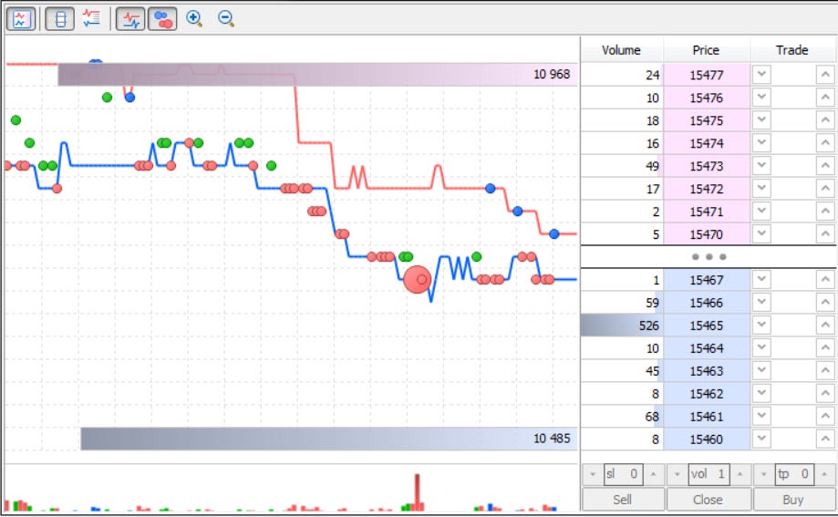
It’s also true that sometimes, if they’re feeling generous, you might even catch a glimpse of the DOM–This is from MT5, probably your broker is receiving this data from contract providers, type CFDs (drama).

Option 2 - Free data–aka the wild west of the Internet:

Next, we have free data—the digital treasure hunt of the quant world. Free data is abundant and comes in many forms: historical price data, economic indicators, and even regulatory filings.

However, it’s a bit like rummaging through a garage sale. Sometimes you find hidden gems, and other times you end up with a box of mismatched, outdated, or poorly formatted information. One must tread carefully in this Wild West of data, where missing values, delayed updates, or bizarre formats might leave you scratching your head—Martian time stamps, anyone?

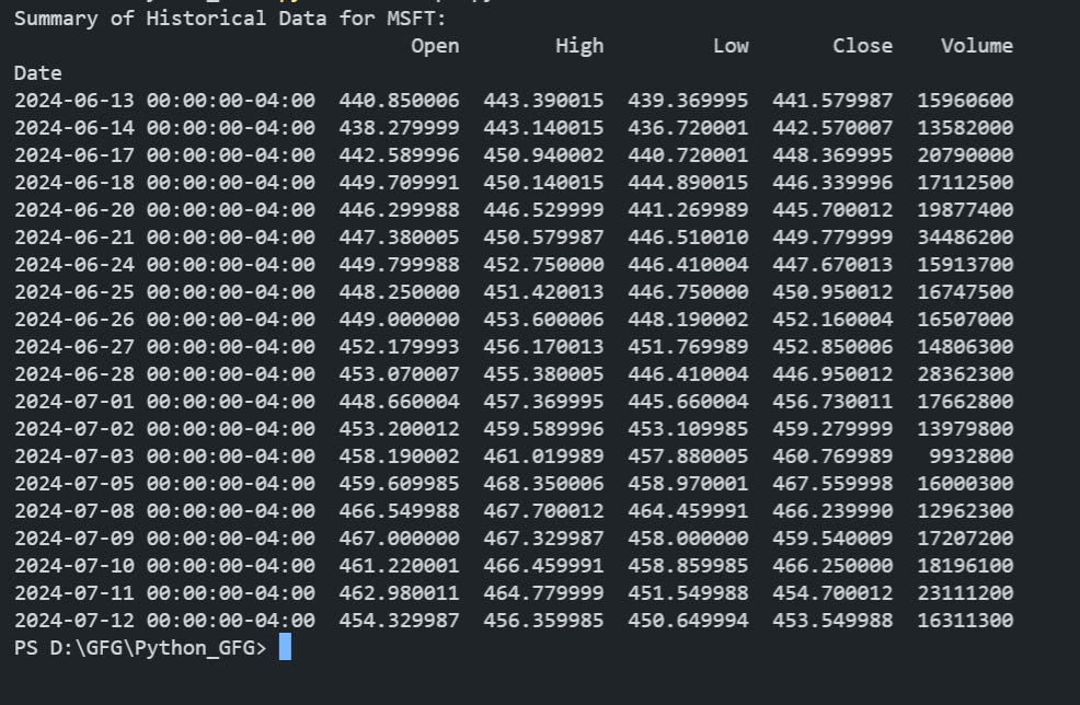
Yes, indeed, I am referring to the infamous Yahoo API:

import yfinance as yf

# Download Tesla stock data from January 1, 2020 to January 1, 2023
data = yf.download("TSLA", start="2020-01-01", end="2025-01-01")
print(data.head())

This snippet is simple, yet effective—unless the data arrives with missing timestamps, delayed or other quirky issues, in which case your cleaning process might soon resemble a detective story with more red herrings than clues.

Option 3 - Paid data–aka the luxury option for retails:

Now, imagine stepping into a high-end boutique, where every product is meticulously curated, and quality is guaranteed—but at a premium price. Paid data is like buying a first-class ticket to data paradise. It offers high-quality, comprehensive datasets that are updated regularly and maintained with rigorous attention to detail. Whether it’s tick-level market data, in-depth fundamental metrics, or alternative datasets, paid data is your golden ticket.

However, be warned: luxury comes at a price and I understand that not everyone can afford it as a hobby. In fact, you might find that the cost of your data is as steep as the learning curve on quantum mechanics–and trust me, that curve is steep!

With paid data, you’re likely to have more accurate predictors, but even then, the model must be validated carefully. After all, as we say in the quant world: garbage in, garbage out—even if the garbage was imported with extra care.

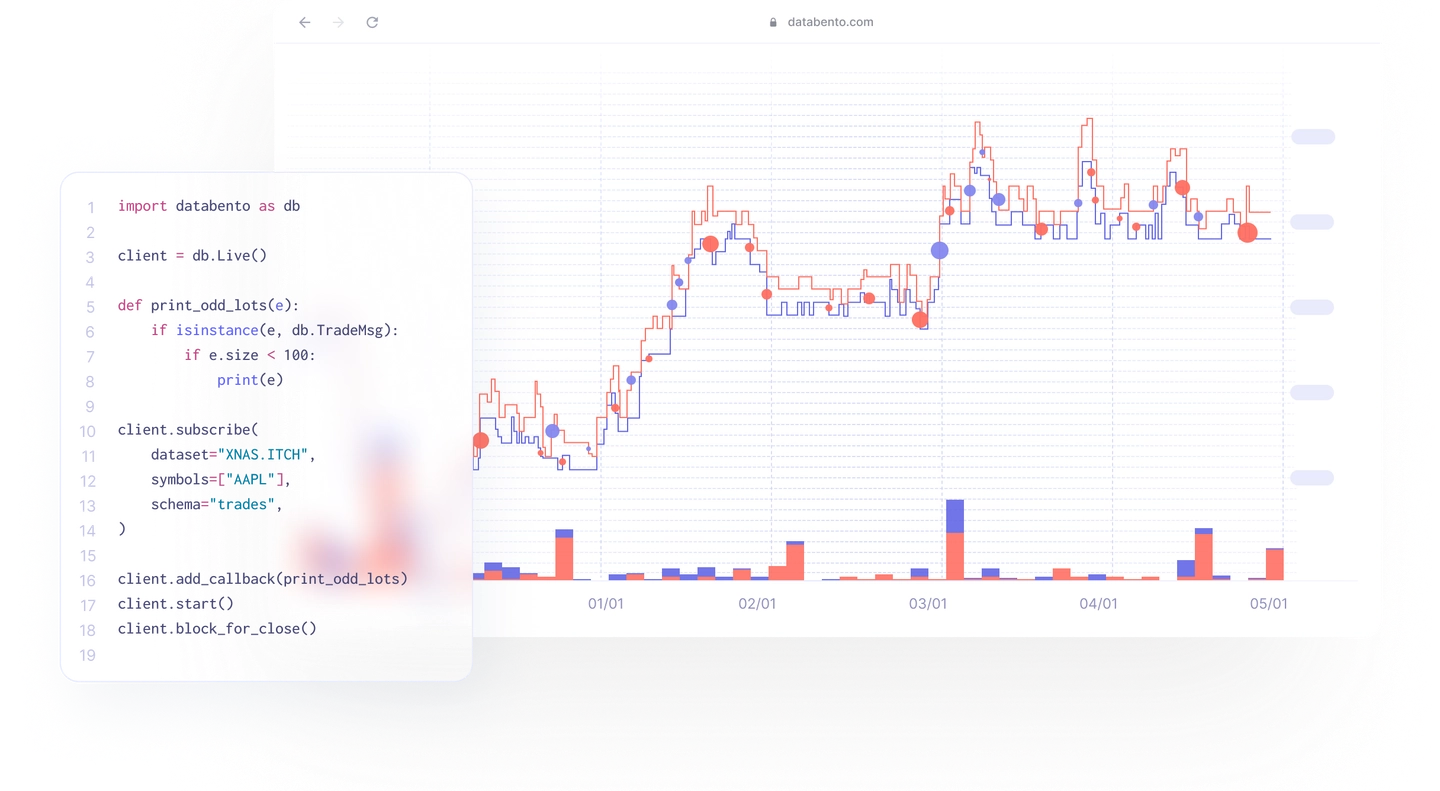
In this case you have this is a sample of Databento, higher quality and better integration.

Option 4 - Data lakes–aka the corporate dream:

Finally, we reach the realm of data lakes—a vast, deep repository where structured, semi-structured, and unstructured data flow together like a mighty river. If you’re part of a large organization, you might have access to a data lake that would make even the most experienced sailor jealous. But for the retail trader, a data lake can feel as unreachable as a private island in the middle of the Atlantic.

In a data lake, you can mix financial statements with multimedia, social media feeds with market data, and even ancient scrolls of economic history–okay, maybe not ancient scrolls, but you get the idea. It’s a corporate dream come true, as long as you have the resources and know-how to swim in its vast depths.

Now that we’ve surveyed the four primary sources of data, let’s move on to the next phase: How to build your own data lake!? It’s time to roll up our sleeves and get our hands dirty with some good old-fashioned data processing!

Building your own mini data lake environment!

Having chosen your data sources, the next logical step is to build an environment where your data can thrive. Whether it’s a sprawling data lake or a modest data pond, the process involves a few key steps: finding data sources, processing your data in batches, ingesting and cleaning it, and finally, storing it in a coherent and efficient manner.

Step 1 - Finding data sources:

The first step in our data episode is akin to assembling a superhero team. You need a diverse set of data sources—financial statements, market valuations, price quotes, news articles, SEC filings, and even social media feeds—to create a robust and versatile dataset. Think of it as building your own Frankenstein’s monster, but instead of cobbling together body parts, you’re stitching together datasets from various origins.

Wait, wait, here comes a good one: Why did the data scientist break up with their dataset? Because it just wasn’t giving them the “connection” they needed! ahaha! Okay, sorry about that. Here some interesting sources:

• iex —free market data.

• one tick—historical tick data.

• iqfeed—real time data feed.

• quantquote—tick and live data.

• algoseek—historical intraday.

• EOD data—historical data.

• intrinio—financial data.

• arctic—igh performance datastore from Man AHL for time series and tick data.

• SEC EDGAR API—query company filings on SEC EDGAR.

The question here is: If I want to take all the sources at once to combine them, how do I do it?

Step 2 - Batch data processing:

Once you have gathered your diverse data sources, it’s time for batch data processing. Imagine doing your laundry: you wait until you have a full load, then wash it all at once. Batch processing is not real-time, but it’s an efficient method for handling large volumes of data at once.

With our batch processing complete, we now have a structured dataset. However, the adventure isn’t over yet. Next, we need to dive into the meticulous process of data ingestion and cleaning—a task that can be as tedious as it is essential.

• Batching: We collect a set of CSV files or other sources and process them all at once.

• Efficiency: By combining them in a single process, we can transform and clean the data in bulk, rather than doing it piecemeal.

• Scalability: Usually, you might be dealing with dozens or hundreds of files, or even streaming these files in daily/hourly batches. The core logic—read, transform, combine—remains the same.

Let’s see an example where we create random dataframes and process them:

import pandas as pd
import numpy as np

class DataBatchProcessor:
    def __init__(self):
        """
        Initialize with:
        - An empty list to hold all DataFrames.
        - A placeholder for the combined DataFrame (initially None).
        """
        self.datasets = []
        self.combined_df = None
        
    def add_dataset(self, df: pd.DataFrame):
        """
        Add a DataFrame to the list of datasets.
        """
        self.datasets.append(df)
    
    def process_datasets(self):
        """
        Combine all individual DataFrames horizontally into a single DataFrame.
        (Columns are placed side-by-side.)
        """
        if self.datasets:
            # Concatenate along axis=1 to place columns side-by-side
            self.combined_df = pd.concat(self.datasets, axis=1)
        else:
            self.combined_df = pd.DataFrame()  # Empty DataFrame if no datasets
    
    def show_all_datasets(self):
        """
        Print all stored DataFrames individually.
        """
        for i, df in enumerate(self.datasets, start=1):
            print(f"Dataset {i}:\n{df}\n{'-'*40}")
            
    def show_combined_dataset(self):
        """
        Print the combined DataFrame.
        """
        if self.combined_df is not None:
            print("Combined DataFrame (horizontally):")
            print(self.combined_df)
        else:
            print("No combined DataFrame found. Please run process_datasets() first.")

def main():
    # Initialize the batch processor
    processor = DataBatchProcessor()
    
    # Create 5 random DataFrames and add them to the processor
    for _ in range(5):
        # Generate random data for a 5x3 DataFrame
        df = pd.DataFrame(
            np.random.randint(0, 100, size=(5, 3)),  
            columns=[f"Col{j+1}" for j in range(3)]
        )
        processor.add_dataset(df)
    
    # Optionally show all individual DataFrames
    processor.show_all_datasets()
    
    # Process: combine all DataFrames horizontally
    processor.process_datasets()
    
    # Show the horizontally combined DataFrame
    processor.show_combined_dataset()

if __name__ == "__main__":
    main()

The previous class only loads and combines dataframes, but here are today's assignments:

• Load data

• Remove duplicates—update the class by adding a function for that.

• Fill missing values—update the class by adding a function for that.

• Displaying results

Leave the output in the comments before continue!—The answer is below.

With our batch processing complete, we now have a cleaner dataset. However, this adventure isn’t over yet. Next, we need to dive into the meticulous process of data ingestion and cleaning—a task that can be as tedious as it is essential.

Step 3 - Data ingestion and cleaning:

Data ingestion is the process of gathering data from various sources and bringing it into your system for further processing. Once the data is ingested, the real work begins: cleaning. This involves removing duplicates, correcting errors, handling missing values, and ensuring the data is formatted uniformly —this would be enough for a complete post, so maybe later.

For the moment, think of it as tidying up your room before your in-laws come to visit—tedious but absolutely necessary.

Let's continue with our toy example. With the previous class, we slightly preprocessed several dataframes; now, it's time to map, clean, and digest:

from sklearn.preprocessing import StandardScaler

class DataCleaner:
    def __init__(self, df: pd.DataFrame):
        """
        Initialize with a DataFrame to clean and preprocess.
        """
        self.df = df.copy()  # Make a copy to avoid modifying the original DataFrame directly
    
    def fill_missing_values(self, value=0):
        """
        Fill any missing (NaN) values in the DataFrame with a given value.
        Default is 0, but can be changed.
        """
        self.df.fillna(value, inplace=True)
    
    def remove_duplicates(self):
        """
        Remove duplicate rows from the DataFrame.
        """
        self.df.drop_duplicates(inplace=True)
    
    def standard_scale_numeric(self):
        """
        Standard-scale (z-score) all numeric columns in the DataFrame.
        (Mean = 0, Std = 1 for each numeric column.)
        """
        numeric_cols = self.df.select_dtypes(include=[np.number]).columns
        scaler = StandardScaler()
        self.df[numeric_cols] = scaler.fit_transform(self.df[numeric_cols])
    
    def get_cleaned_data(self):
        """
        Return the cleaned/preprocessed DataFrame.
        """
        return self.df

def main():
    # 1. Initialize the batch processor
    processor = DataBatchProcessor()
    
    # 2. Create 5 random DataFrames and add them to the processor
    for _ in range(5):
        # Generate random data for a 5x3 DataFrame
        df = pd.DataFrame(
            np.random.randint(0, 100, size=(5, 3)),  
            columns=[f"Col{j+1}" for j in range(3)]
        )
        processor.add_dataset(df)
    
    # Optionally show all individual DataFrames
    processor.show_all_datasets()
    
    # 3. Combine all DataFrames horizontally
    processor.process_datasets()
    
    # 4. Show the combined DataFrame before cleaning
    processor.show_combined_dataset()
    
    # 5. Create a DataCleaner with the combined dataset
    cleaner = DataCleaner(processor.combined_df)
    
    # 6. Perform some cleaning/preprocessing
    cleaner.fill_missing_values(value=0)  # fill NaNs with 0 if any exist
    cleaner.remove_duplicates()           # remove duplicate rows if any
    cleaner.standard_scale_numeric()      # standard-scale all numeric columns
    
    # 7. Retrieve and display the cleaned DataFrame
    cleaned_df = cleaner.get_cleaned_data()
    print("\nCleaned & Preprocessed DataFrame:")
    print(cleaned_df)

if __name__ == "__main__":
    main()

Apart from cleaning, you can transform your data with:

• Mathematical transformations.

• Structural transformations.

• Geometric transformations.

• Text data transformations.

• Dimensionality reduction.

• Encoding & feature engineering.

• Temporal transformations.

At this point, you've wrestled with missing values, cleaned up duplicate entries, and even tamed a few rogue outliers. Congratulations! Your dataset is finally looking respectable—dare I say, presentable. But before you pop the champagne, there's one more crucial step: storing your data in a way that doesn’t turn your future self into a detective hunting for missing files.

Step 4 - Data storage:

After the data has been ingested and cleaned, the final step in this phase is storing it in a structured and accessible way. Proper data storage involves partitioning the data by time frames or asset classes, indexing it for quick retrieval, and implementing security measures to protect sensitive information. Think of it as organizing your library: you wouldn’t want to mix mystery novels with science textbooks, would you?

Proper organization not only makes data retrieval efficient but also lays the foundation for subsequent analysis and modeling. A well-organized database is like a well-organized closet—everything has its place, and you can find that missing sock (or in our case, a crucial data point) in no time.

Now that we’ve gathered, processed, and stored our data, it’s time to add a little extra magic—metadata and data mapping. These final touches are essential for understanding the intricate details of your data and preparing it for the modeling phase.

And just like that, we’ve conquered the first half of our quant adventure. We’ve journeyed through the tangled jungle of data sourcing, navigated the treacherous waters of data cleaning, and emerged victorious with a dataset that is well-structured, mapped, and labeled with precision. If data were a chaotic puzzle, we’ve now assembled the edges and sorted the pieces by color—ready for the masterpiece to take shape.

But, dear reader, our journey doesn’t end here. The real magic begins when we take this beautifully structured data and breathe life into it with mathematical models. That’s where we move from data wrangling to quantitative reasoning, from organization to prediction, from raw numbers to meaningful insights.

However, that’s a story for another day. For now, take a moment to appreciate how far we’ve come. Your dataset is no longer a wild, unstructured mess—it’s a refined, intelligent repository ready for the next stage of its evolution.

So, take a break, grab a coffee, and prepare yourself for our next adventure: applying mathematical models to turn structured data into actionable insights. Because when numbers start talking, the real fun begins.

Until next time—happy quanting! 🚀📈

---

👍 Did you gain valuable insights and now want to empower others in the field?

---

Appendix
If you want to learn more about data lakes, here’s a guide:

Essential Guide To Data Lakes Designing Data Lakes To Optimize Analytics

571KB ∙ PDF file

Download

Download