[WITH CODE] Features: Incremental feature selection
Introducing the fully automated incremental OMP methodology
Table of contents:
Introduction.
Classical Orthogonal Matching Pursuit.
Fully automated incremental OMP.
Incremental QR update.
Robust noise estimation via MAD.
Z‑Score normalization for non‑stationarity.
FA-OMP incremental algorithm implementation.
Introduction
Who doesn't use a feature selection method? Questions here, feature this, and blah blah blah, questions there, and feature this, and lalala. Well, let's look at a rather interesting technique. The original method has quite a few flaws, but many of them have been eliminated with today’s implementation. I’m refering to the Orthogonal Matching Pursuit method.
This type of method have long been used in compressed sensing and signal processing, but classical OMP is known to suffer from pitfalls like greediness, sensitivity to noise, and high computational costs.
But first things first, let's see an introduction of the class method and then the improved version.
Classical Orthogonal Matching Pursuit
In order to understand it we have to take into account the sparse representations and the ℓ₀-norm.
So given an observation vector
and a dictionary
we assume that y can be expressed as
where w∈RN is a sparse coefficient vector—i.e., it has only a few nonzero entries—and e represents noise. The sparsity of w is often measured using the so-called ℓ₀-norm:
Finding the sparsest solution is NP‑hard, which motivates the use of greedy algorithms.
So what does this technique consist of? It is a iterative algorithm that selects one dictionary atom at a time. At each iteration t, OMP computes the residual
where Λt-1 is the set of indices selected so far. The next atom is chosen as
After adding the new atom, the algorithm updates the coefficient vector wΛt by solving the least-squares problem:
You can check it by using this snippet:
import numpy as np
import matplotlib.pyplot as plt
from sklearn.linear_model import OrthogonalMatchingPursuit
# Set a random seed for reproducibility
rng = np.random.RandomState(42)
# -------------------------------------------------------
# 1. Generate synthetic data
# -------------------------------------------------------
n_samples = 40 # Number of samples
n_features = 100 # Number of features (dictionary atoms)
n_nonzero_coefs = 5 # True number of nonzero coefficients
# Design matrix (dictionary)
X = rng.randn(n_samples, n_features)
# True (sparse) coefficients
w_true = np.zeros(n_features)
# Randomly pick positions for the nonzero coefficients
idx = rng.choice(np.arange(n_features), n_nonzero_coefs, replace=False)
# Assign random values to these positions
w_true[idx] = rng.randn(n_nonzero_coefs)
# Generate target values
y = X @ w_true
# -------------------------------------------------------
# 2. Fit Orthogonal Matching Pursuit
# -------------------------------------------------------
omp = OrthogonalMatchingPursuit(n_nonzero_coefs=n_nonzero_coefs)
omp.fit(X, y)
# Recovered coefficients
w_estimated = omp.coef_
If we plot this, we get:
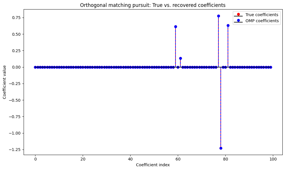
The plot shows both the true coefficients and the ones recovered by OMP.
Despite its simplicity, classical OMP suffers from:
Early incorrect selections are irreversible, potentially leading to suboptimal global performance.
Noise can distort correlation measurements, resulting in the selection of irrelevant atoms.
Repeatedly solving full least-squares problems is expensive.
Manual tuning is needed for thresholds and stopping criteria.
At the beginning my goal was to address these issues through automation, incremental updates and robust noise estimation. But as I solved one problem, another appeared. Until I was finally able to establish a method.
Fully automated incremental OMP
There are several points that have had to be changed a priori if the goal is to achieve an incremental release. Let's start with the first one.
Incremental QR update
Suppose that after k iterations we have the selected sub-dictionary XΛt with its QR decomposition:
where Q∈RM×k is an orthonormal matrix and R∈Rk×k is upper-triangular. When a new atom a is added, we wish to efficiently compute the QR decomposition of the augmented matrix
We first project a onto Q:
and compute the residual
Its norm is
If rnorm is significant, we form
and update the basis:
and the upper-triangular factor becomes:
This update is encapsulated in our helper function incremental_qr_update
. As we will see in the final version.
Let’s put this into code:
import numpy as np
import matplotlib.pyplot as plt
def incremental_qr_update(Q, R, a):
"""
Incrementally update the QR decomposition when adding a new column a.
Given Q (M x k) and R (k x k) such that A = Q @ R, where A consists of
previously selected atoms, compute the QR of [A, a].
"""
p = Q.T @ a # Projection of a onto Q, shape (k,)
r_vec = a - Q @ p # Residual component of a
r_norm = np.linalg.norm(r_vec)
if r_norm < 1e-12:
# Nearly in the span of Q; avoid division by zero.
r_norm = 1e-12
new_col = np.zeros_like(a)
else:
new_col = r_vec / r_norm
Q_new = np.column_stack([Q, new_col])
R_new_top = np.column_stack([R, p.reshape(-1, 1)])
R_new_bottom = np.zeros((1, R.shape[1] + 1))
R_new_bottom[0, -1] = r_norm
R_new = np.vstack([R_new_top, R_new_bottom])
return Q_new, R_new
Robust noise estimation via MAD
Classical OMP requires an estimate of the noise standard deviation σ. In non‑stationary environments like trading, a fixed noise estimate can be misleading. We therefore adopt a robust noise estimation technique using the median absolute deviation of the residual:
and approximate
This robust estimate updates as the algorithm proceeds and is used to adapt the correlation threshold dynamically. 0.6745 is constant used for normal distributions—remember that we will normalize our data with the next step.
That’s easy!
def robust_noise_estimation(residual):
"""
Estimate noise standard deviation robustly using the Median Absolute Deviation (MAD).
"""
med = np.median(residual)
mad = np.median(np.abs(residual - med))
sigma = mad / 0.6745 # Constant for normal distribution
return sigma
Z‑Score normalization for non‑stationarity
To address non‑stationarity, we preprocess the dictionary X by converting each column into its z‑score:
where μj and σj are the mean and standard deviation of the j‑th column. This transformation ensures that features are standardized, thus making the correlation comparisons more reliable over time.
FA-OMP incremental algorithm implementation
Even with backtracking, the greedy nature of OMP might cause suboptimal early selections. To mitigate this, we need to introduce a greedy swap procedure. After updating the residual, if the relative improvement is insufficient, the algorithm iterates over each selected atom and checks whether replacing it with a candidate—from those not yet selected—improves the residual significantly. If a beneficial swap is found, the algorithm replaces the atom and updates the QR decomposition accordingly.
Oka! Time to implement final part of this procedure!
def fully_automated_omp_incremental_improved(X, y, max_atoms=20, init_lambda=1e-3,
auto_lambda=True, cond_threshold=1e6,
init_corr_threshold_factor=3,
max_threshold_adapt=5, backtrack=True,
rel_improve_tol=1e-3, max_no_improve_iter=3,
use_zscore=True, update_noise=True, greedy_swap=True):
"""
Fully Automated Incremental OMP (FA-OMP) with additional improvements:
- Z-score normalization for non-stationarity.
- Robust noise estimation (using MAD) to update noise_std.
- Greedy swap procedure to mitigate early selection pitfalls.
Returns:
w: Recovered coefficient vector (N,)
selected_indices: List of selected atom indices.
residuals: List of residual norms at each iteration.
"""
M, N = X.shape
# Preprocess: use z-score normalization if requested.
if use_zscore:
X_z = np.zeros_like(X)
for j in range(N):
col = X[:, j]
mu = np.mean(col)
sigma = np.std(col)
sigma = sigma if sigma > 1e-12 else 1.0
X_z[:, j] = (col - mu) / sigma
X_norm = X_z.copy()
else:
# Simple normalization by column norm.
col_norms = np.linalg.norm(X, axis=0)
col_norms[col_norms == 0] = 1
X_norm = X / col_norms
# Initial robust noise estimation if update_noise is enabled.
if update_noise:
noise_std = robust_noise_estimation(y)
else:
noise_std = 0.05
r = y.copy()
selected_indices = []
residuals = [np.linalg.norm(r)]
# For incremental update, maintain Q and R for the selected sub-dictionary.
Q = None
R = None
corr_threshold_factor = init_corr_threshold_factor
current_lambda = init_lambda
no_improve_count = 0
prev_res_norm = residuals[-1]
for t in range(max_atoms):
# Optionally update noise estimation from the current residual.
if update_noise:
noise_std = robust_noise_estimation(r)
# Compute correlations with normalized dictionary atoms.
correlations = X_norm.T @ r
abs_corr = np.abs(correlations)
# Adaptive thresholding: relax threshold if no candidate qualifies.
adapt_count = 0
valid_indices = np.where(abs_corr >= corr_threshold_factor * noise_std)[0]
while valid_indices.size == 0 and adapt_count < max_threshold_adapt:
corr_threshold_factor *= 0.8
valid_indices = np.where(abs_corr >= corr_threshold_factor * noise_std)[0]
adapt_count += 1
if valid_indices.size == 0:
print("No valid atom found after adaptive thresholding. Stopping.")
break
# Sort valid indices by descending correlation.
sorted_valid = valid_indices[np.argsort(-abs_corr[valid_indices])]
candidate_found = False
for candidate in sorted_valid:
if candidate not in selected_indices:
new_atom = candidate
candidate_found = True
break
if not candidate_found:
print("All valid atoms have been selected. Stopping.")
break
selected_indices.append(new_atom)
a = X_norm[:, new_atom]
# Incrementally update Q and R.
if Q is None:
norm_a = np.linalg.norm(a)
norm_a = norm_a if norm_a >= 1e-12 else 1e-12
Q = a.reshape(-1, 1) / norm_a
R = np.array([[norm_a]])
else:
Q, R = incremental_qr_update(Q, R, a)
# Compute least-squares solution via incremental QR.
w_sel = np.linalg.solve(R, Q.T @ y)
# Fallback: if R is ill-conditioned, increase lambda and recalc.
cond_number = np.linalg.cond(R)
if auto_lambda and cond_number > cond_threshold:
current_lambda *= 10
print(f"Increasing lambda due to high condition number: {cond_number:.2e}")
X_sel = X_norm[:, selected_indices]
A_aug = np.vstack([X_sel, np.sqrt(current_lambda) * np.eye(len(selected_indices))])
y_aug = np.concatenate([y, np.zeros(len(selected_indices))])
w_sel, _, _, _ = np.linalg.lstsq(A_aug, y_aug, rcond=None)
Q, R = np.linalg.qr(X_sel, mode='reduced')
# Compute approximation and new residual.
y_est = Q @ (R @ w_sel)
new_r = y - y_est
new_res_norm = np.linalg.norm(new_r)
residuals.append(new_res_norm)
# Check for relative improvement.
rel_improve = abs(prev_res_norm - new_res_norm) / (prev_res_norm + 1e-12)
if rel_improve < rel_improve_tol:
no_improve_count += 1
else:
no_improve_count = 0
prev_res_norm = new_res_norm
if no_improve_count >= max_no_improve_iter:
print("No significant improvement for several iterations. Stopping.")
break
# Automated backtracking: remove any atom whose removal improves the residual.
if backtrack and len(selected_indices) > 1:
improvement = True
while improvement:
improvement = False
for idx in selected_indices.copy():
temp_indices = selected_indices.copy()
temp_indices.remove(idx)
if not temp_indices:
continue
X_temp = X_norm[:, temp_indices]
Q_temp, R_temp = np.linalg.qr(X_temp, mode='reduced')
w_temp = np.linalg.solve(R_temp, Q_temp.T @ y)
r_temp = y - Q_temp @ (R_temp @ w_temp)
if np.linalg.norm(r_temp) < new_res_norm * (1 - rel_improve_tol):
print(f"Backtracking: removed atom {idx} for improvement.")
selected_indices = temp_indices
new_r = r_temp
new_res_norm = np.linalg.norm(r_temp)
w_sel = w_temp
residuals[-1] = new_res_norm
Q, R = np.linalg.qr(X_norm[:, selected_indices], mode='reduced')
improvement = True
break
# Greedy swap procedure: try to replace one selected atom with a candidate not selected.
if greedy_swap and len(selected_indices) > 1:
for idx in selected_indices.copy():
for candidate in sorted_valid:
if candidate in selected_indices:
continue
temp_indices = selected_indices.copy()
temp_indices[temp_indices.index(idx)] = candidate
X_temp = X_norm[:, temp_indices]
Q_temp, R_temp = np.linalg.qr(X_temp, mode='reduced')
w_temp = np.linalg.solve(R_temp, Q_temp.T @ y)
r_temp = y - Q_temp @ (R_temp @ w_temp)
if np.linalg.norm(r_temp) < new_res_norm * (1 - rel_improve_tol):
print(f"Greedy swap: replacing atom {idx} with {candidate} for improvement.")
selected_indices = temp_indices
new_r = r_temp
new_res_norm = np.linalg.norm(r_temp)
w_sel = w_temp
residuals[-1] = new_res_norm
Q, R = np.linalg.qr(X_norm[:, selected_indices], mode='reduced')
break
r = new_r
if new_res_norm < noise_std:
print("Residual norm below noise level. Stopping.")
break
# Final coefficient vector (undo z-score if used).
w = np.zeros(N)
if selected_indices:
if use_zscore:
# For z-score normalized columns, coefficients represent standardized effects.
w[selected_indices] = w_sel
else:
# Undo normalization by dividing by original column norms.
col_norms = np.linalg.norm(X, axis=0)
col_norms[col_norms == 0] = 1
w[selected_indices] = w_sel / col_norms[selected_indices]
return w, selected_indices, residuals
This algorithm helps extract a small subset of significant predictors from a large pool. So let’s test it 🤓
# Simulated Trading Feature Selection Example
import numpy as np
import matplotlib.pyplot as plt
np.random.seed(123)
M = 200 # Number of days
N = 50 # Candidate features
true_k = 5
# Generate simulated feature matrix
X_trading = np.random.randn(M, N)
# Construct a sparse true coefficient vector
w_true_trading = np.zeros(N)
true_feature_indices = np.random.choice(range(N), true_k, replace=False)
w_true_trading[true_feature_indices] = np.random.randn(true_k)
# Simulate observed returns with noise
noise_std_trading = 0.1
noise_trading = noise_std_trading * np.random.randn(M)
y_trading = X_trading @ w_true_trading + noise_trading
# Apply the improved FA-OMP incremental algorithm
max_atoms_trading = 15
w_est_trading, selected_indices_trading, residuals_trading = fully_automated_omp_incremental_improved(
X_trading, y_trading, max_atoms_trading, init_lambda=1e-3, auto_lambda=True,
cond_threshold=1e6, init_corr_threshold_factor=3, max_threshold_adapt=5,
backtrack=True, rel_improve_tol=1e-3, max_no_improve_iter=3, use_zscore=True,
update_noise=True, greedy_swap=True
)
print("True feature indices:", true_feature_indices)
print("Recovered feature indices:", selected_indices_trading)
With this snippet you get the indexes of the features you need to choose. And if you plot the above simulation you get this:
The plot tells us that the algorithm quickly finds the most critical features to explain the returns, and after a certain point, additional features don't provide significant benefits.
Alright folks, that’s a wrap for today! Catch you next time—keep exploring, trade with purpose, and let the data do the talking! 📊✨
PS: Are you exploring blockchain or DeFi methods for algo trading?
Appendix
If you want to know more about the original method, check this: