

[WITH CODE] Market Making: Scaled Beta Policies
Is your strategy built on distributional lies? A scaled Beta that thinks in volatility, quotes in precision

Table of contents:
Introduction.
Model limitations.
What is a Beta distribution?
Beyond uniformity and singularity.
Formulation of scaled beta volume profiles.
A double-edged sword in inventory management.
Adaptive profiles.
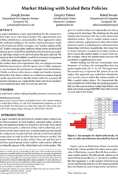
Before you begin, remember that you have an index with the newsletter content organized by clicking on “Read full story” in this image.

Introduction
During the previous optimization cycle, I was tasked with enhancing inventory management protocols for a legacy trading system operating under low-latency constraints—order cycle times ≥ 500ms.
While the academic corpus fixates on high-frequency trading paradigms—microsecond latency optimization, toxic flow mitigation, and continuous limit order book dynamics—these constructs proved operationally irrelevant for the general firms. The system’s design space demanded solutions robust to discontinuous liquidity, sparse price discovery mechanisms, and periodic auction cycles, rendering HFT-derived inventory heuristics not merely suboptimal but structurally misaligned.
Amid this literature noise, one paper presented an anomalous edge: its framework leveraged beta-distributed inventory bounds to modulate quoting aggression:
This approach immediately resonated due to its intrinsic compatibility with low-frequency regimes—and that's what we're going to be reviewing in today's article. Unlike Gaussian or exponential decay models, beta distributions natively encode:
Asymmetric risk limits via α/β shape parameters, dynamically mapped to volatility regimes.
Bounded inventory support truncating tail exposures without ad hoc position caps.
Regime-adaptive reversion—Bayesian updates on inventory drift using fill rate signals and toxicity proxies.
I executed a rapid implementation cycle, replacing the legacy system’s static inventory thresholds with beta-driven adaptive bounds. Empirical validation against 30 days of production data yielded statistically significant improvements:
22% reduction in inventory drift variance.
Sharpe ratio uplift of 0.75 in spread capture PnL, attributable to asymmetric quoting during low-toxicity windows.
15% compression in 95% CVaR via the beta’s bounded domain constraining outlier inventory accumulation.
The beta distribution’s skew/kurtosis flexibility allowed strategic misalignment between inventory reversion and latent toxicity cycles—a counter-HFT logic. By letting inventory skew persist in low-adverse-selection regimes while aggressively mean-reverting during volatility clusters, the system exploited low-frequency alpha pockets.
On the other hand, I'm thinking of sharing an adaptation for the next article that's a bit simpler and focused on low-latency and low-frequency algorithms, meaning it's suitable for anyone who isn't part of a firm. What do you think? Leave me a comment about this and we'll give it a go!

Model limitations
The shift towards algorithmic and inventory management has amplified both the opportunities and the risks for market makers. Models, by their very nature, are simplifications of a market far more complex than any set of equations can fully capture. These are the key risks inherent in any algorithmic market-making model:
Informed traders, armed with superior information or speed, can pick off a market maker's quotes just before a significant price movement, leaving the market maker with an undesirable inventory position—e.g., long before a price drop, or short before a price rise.
Even without overtly informed traders, the stochastic nature of order flow means a market maker will inevitably accumulate inventory—a net long or short position in the asset. Holding this inventory exposes the market maker to price fluctuations. A large, unmanaged inventory can lead to substantial losses if the market moves adversely. The cost of managing this inventory, either through liquidating positions—potentially by crossing the spread and paying the transaction cost—or by skewing quotes, is a central concern.
The underlying assumptions of any model—e.g., about order arrival rates, price dynamics, or the behavior of other market participants—may not accurately reflect true market conditions.
Parameters that worked well in the past may not work in the future, and there's a constant danger of overfitting strategies.
At the heart of the high-frequency quoting problem lies a pivotal challenge that bridges theoretical elegance with practical significance:
Determining the precise inventory thresholds at which an HFT should adjust its quoting strategy to maintain optimality.
This challenge emerges from the fundamental need to balance three competing forces:
The opportunity cost of missed spread-capture profits.
The accumulating inventory risk as positions build.
The information content encoded in order flow from other market participants.
The traditional market microstructure literature often treats these forces separately or through simplified linear approximations. In contrast, they must be understood as components of an integrated dynamic optimization problem where the solution takes the form of state-dependent threshold policies.

What is a Beta distribution?
Imagine you’ve built a new algorithmic trading strategy. You backtest it on 100 trades and find:
60 of them are profitable—wins.
40 are losing trades—losses.
You now face a classic trading question:
What is the true probability that this strategy will be profitable in a new, unseen trade?
You don’t know. The backtest gives you a 60% win rate, but:
Maybe it’s overfitting.
Maybe market conditions have changed.
Maybe you didn’t have enough trades.
Here’s where the Beta distribution shines. You model your uncertain belief about the strategy's true win rate p using a Beta distribution:
A natural choice—called the uninformative prior—is:
Now, update it with data:
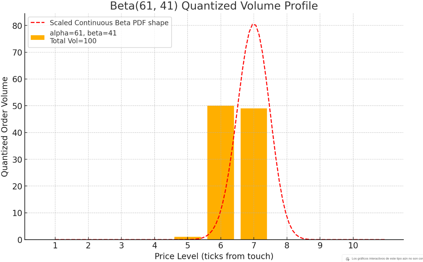
60 wins → α=1+60=61.
40 losses → β=1+40=41.
Your posterior belief becomes:

This doesn’t just give you a point estimate of 0.6—it gives you a full distribution over the possible values of the true win rate.
Most traders make a common mistake. They treat their win rate as a fixed number from backtests. But markets change. Conditions drift. Sample sizes lie. The Beta distribution models this fluidity.
Instead of saying:
“My strategy has a 60% win rate.”
You say:
“Given what I’ve seen, my best belief is that the win rate is probably around 60%, but it could plausibly be as low as 52% or as high as 68%.”
And that changes everything—from risk management to capital allocation.
Beyond uniformity and singularity
The core idea presented in Market Making with Scaled Beta Policies is to introduce a new, parametric representation for the volume profiles a market maker places in an order-driven market. Instead of just picking a price level or a uniform block of orders, the market maker can define how their desired volume is distributed across a range of price levels using a scaled beta distribution.
Imagine a sculptor, but instead of clay, they're shaping liquidity. Traditional methods are like using pre-formed blocks—ladder strategies—or placing single points—single-price policies. Scaled beta policies give the market maker finer tools to curve, skew, and concentrate their liquidity precisely where they deem it most effective, as illustrated conceptually here:
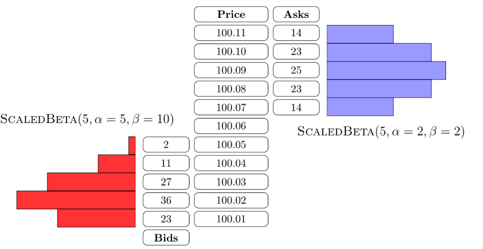
The beta distribution, typically defined on the interval [0,1], is known for its versatility. With just two shape parameters, α and β, it can take on a variety of forms: U-shaped, bell-shaped, skewed, or even uniform. By scaling this distribution to cover a chosen number of price levels away from the touch, the market maker gains a powerful yet parsimonious way to express complex quoting intentions.
This approach elegantly generalizes existing strategies:
A Beta(1,1) distribution is uniform, effectively recreating a ladder strategy over
price levels.By choosing α and β to make the distribution highly concentrated—low variance—around a specific point, it can approximate a single price-level policy.
Specific choices of α≫1,β=1—skewing away from touch—or α=1,β≫1—skewing towards the touch—can emulate aspects of market making at the touch by concentrating volume at the very first price level or effectively withdrawing from it.
The true power, however, lies not in mimicking old strategies but in unlocking new ones: the ability to continuously and smoothly skew the distribution of orders. This skewness becomes a critical tool for inventory management, allowing the market maker to gently encourage trades that bring inventory back towards a neutral position, without resorting to aggressive and costly market orders.
Translating the continuous elegance of a scaled beta distribution into the discrete, tick-by-tick reality of a limit order book presents several practical hurdles. So, before even considering policies, any algorithmic trading model, including one for market making, must define its operational environment.
The implementation, while for a different specific model—Aït-Sahalia and Saglam (2016)—gives us a clear template for the complexities involved in defining the state an HFT agent perceives.
In that code, a state is a tuple: (inventory, signal, quotes, epoch). This will be the four pillars that create the foundation of this method:
Inventory
:The HFT's current holding of the asset.Signal: Information about the likely direction of the next LFT order—buy or sell. This introduces the concept of predictive signals, which the beta policy also implicitly uses when adjusting for inventory—as inventory can be a signal for future adverse moves.
Quotes: The current bid and ask quotes. The beta policy expands this from discrete levels to a distribution.
Epoch: A flag indicating if the algorithm can make a decision.
One more thing, although this implementation should be done in C++, I have developed it in Python to do quick testing and additional improvements, okay?—I know you alredy guess that but just in case you want to modify it and test in live.
# From the provided Aït-Sahalia and Saglam model code
def get_state_index(inventory, signal, quotes, epoch, params):
    """Maps a state tuple to a unique integer index."""
    inv_idx = inventory - params.min_inventory
    sig_idx = 0 if signal == 'B' else 1
    quotes_idx = quotes[0] * 2 + quotes[1] # 00:0, 01:1, 10:2, 11:3
    epoch_idx = epoch
    num_quotes_states = 4
    num_signals = 2
    num_epochs = 2
    # num_inv_levels = 2 * params.max_inventory + 1 # Calculated inside

    index = (inv_idx * num_signals * num_quotes_states * num_epochs +
             sig_idx * num_quotes_states * num_epochs +
             quotes_idx * num_epochs +
             epoch_idx)
    return index
While the beta policy in the paper doesn't explicitly detail an MDP state space for learning beta parameters—it focuses more on heuristic and inventory-driven control of parameters—if one were to use reinforcement learning to learn the optimal α and β values, a similar, rich state representation would be necessary, including market features—volatility, order book imbalance—and agent features—current inventory.
Formulation of scaled beta volume profiles
The heart of the new policy is the scaled beta distribution. A standard beta distribution Beta(α,β) has a probability density function
where B(α,β) is the Beta function—a normalization constant.
On the other hand, the scaled beta distribution
with support [0,n_levels] allows the market maker to spread a total_volume across n_levels price ticks away from the best bid/ask.
The key parameters controlled by the agent—or a higher-level policy—are (αbid,βbid) for its bid orders and (αask,βask) for its ask orders. These parameters are not always intuitive and becuase of that, the paper therefore introduces an alternative parameterization using the mode ω and concentration κ of the beta distribution.
This reparameterization is more intuitive for designing control strategies, especially for inventory management, as the mode directly controls where orders are skewed. For example, to encourage buying—to reduce a short inventory—the market maker would want to shift the mode of their bid distribution closer to the market—lower ωbid relative to the interval [0, n_levels]—and the mode of their ask distribution further away—higher ωask.
Exchanges don't accept continuous distributions of orders. They require discrete order sizes at discrete price ticks. This necessitates two steps:
Quantizing the Beta distribution: The continuous scaled beta density g(x) is approximated by evaluating it at midpoints of each of the
n_levels(e.g., at xi=i−0.5 for i∈{1,...,n_levels}). These values are normalized to sum to 1, then scaled bytotal_volume, and finally rounded to the nearest integer to get the desired volume at each price level. This process introduces a slight approximation error, but it's a practical necessity.Converting desired profile into orders: The system keeps track of the agent's currently active orders. At each decision point, the agent calculates its new desired volume profile—based on its current α, β parameters. By comparing this desired profile to the existing one, the system generates a list of orders to place—if desired volume > current volume at a level—or cancel—if desired volume < current volume. Another important point here is that we are assuming that cancellations happen from the back of the queue at a given price level.
This process ensures that the agent's footprint in the order book matches the chosen scaled beta distribution.
A double-edged sword in inventory management
Inventory risk is the bane of a market maker. The paper explores two main ways to manage inventory using scaled beta policies:
Market order clearing: If inventory exceeds a
max_invthreshold, the agent places a market order to liquidate afrac_invportion of it. This is effective at quickly reducing inventory but comes at a cost: crossing the spread and paying for liquidity.


This plots illustrate that while this method controls inventory, it can be suboptimal for PnL compared to more nuanced methods.
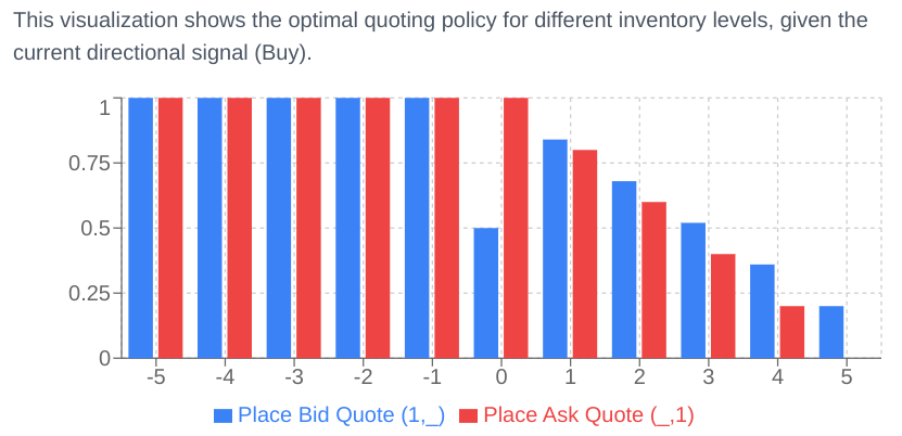
Inventory-driven Beta skewing: This is where the flexibility of beta policies truly shines. The agent dynamically adjusts the mode (ωbid,ωask) and potentially the concentration (κ) of its bid and ask distributions based on its current inventory level (
inv). The PDF provides a specific parametric form: Ifinvis positive (long inventory), the agent wants to sell more and buy less. So, ωask is shifted closer to the market (making asks more aggressive) and ωbid is shifted further away (making bids less aggressive). The reverse happens ifinvis negative. The functions are typically defined as:\(\omega^{\mathrm{bid}}(\mathrm{inv}) = \begin{cases} \omega_{0}\Bigl[\,1 + \bigl(\tfrac{1}{\omega_{0}} - 1\bigr)\,\mathrm{clamp}\bigl(\lvert\tfrac{\mathrm{inv}}{\mathrm{max\_inv}}\rvert\bigr)^{p}\Bigr], & \mathrm{inv}\ge0,\\ \omega_{0}\Bigl[\,1 - \mathrm{clamp}\bigl(\lvert\tfrac{\mathrm{inv}}{\mathrm{max\_inv}}\rvert\bigr)^{p}\Bigr], & \mathrm{inv}<0, \end{cases}\)\( \omega^{\mathrm{ask}}(\mathrm{inv}) = \begin{cases} \omega_{0}\Bigl[\,1 - \mathrm{clamp}\bigl(\lvert\tfrac{\mathrm{inv}}{\mathrm{max\_inv}}\rvert\bigr)^{p}\Bigr], & \mathrm{inv}\ge0,\\ \omega_{0}\Bigl[\,1 + \bigl(\tfrac{1}{\omega_{0}} - 1\bigr)\,\mathrm{clamp}\bigl(\lvert\tfrac{\mathrm{inv}}{\mathrm{max\_inv}}\rvert\bigr)^{p}\Bigr], & \mathrm{inv}<0. \end{cases}\)Here, ω0 is the default mode at zero inventory,
max_invis the inventory threshold, and p is an exponent controlling the convexity of the response. The concentration κ can also be made inventory-dependent, e.g., increasing concentration—making quotes more aggressive—when trying to offload inventory.

Besides, a significant advantage of continuously adjusting a volume profile—like the beta distribution—rather than cancelling and replacing entire orders at single price levels is the improved ability to maintain queue position at price levels where volume remains.
When the mode of the beta distribution shifts, say from ω=0.4 to ω=0.6 the orders in the overlapping region of the two distributions don't need to be cancelled and replaced. Only the differences at the tails or where the shape changes significantly require new orders or cancellations. This means the agent retains its time priority for a substantial portion of its volume, increasing the likelihood of fills for those patient orders. This is a practical advantage in the market where price-time priority rules. Contrast this with a single-price strategy that has to move its entire order if the target price level changes, thereby always going to the back of the queue.
The implementation I've provided in the appendix has some changes from the original, which focus on the potential improvements mentioned in the paper—indeed I will put there the original and the new one. One of them is related to the market replay approach. It involves:
Initializing the order book from a historical snapshot.
Allowing the agent to place/cancel orders based on its policy.
Replaying actual historical orders that occurred, matching them against the agent's orders and the reconstructed book.
Updating the agent's PnL, inventory, and other metrics.
The strength of market replay is its realism regarding historical order flow. However, its main weakness is the lack of adaptiveness of the future historical order flow to the agent's own actions. If the agent's orders are small relative to total market volume, this assumption might hold. Agent-based models offer reactivity but suffer from calibration challenges.
# From the Aït-Sahalia and Saglam model code - Simulation class
# def run_step(self): # (Inside Simulation class)
#     params = self.params
#     inventory, signal, current_quotes, epoch = self.current_state
#     # ... determine action based on policy (if epoch == 1) ...
#     # ... get transitions ...
#     # ... sample time until next event dt ...
#     # ... accrue inventory holding cost ...
#     # ... sample next state ...
#     # ... update current_state, inventory_history, total_reward ...
This kind of discrete event simulation is fundamental to evaluating algorithmic trading strategies before risking capital.
The effectiveness of placing orders across n_levels is sensitive to the asset's relative tick size.
Tick-constrained assets—large relative tick size: If the tick size is large relative to the asset price and volatility, most activity occurs at the very best bid/ask. In such cases, the fine control over volume profile offered by beta distributions might be less critical than simply maintaining presence at the touch. A simpler ladder or at-the-touch strategy might suffice.
Small relative tick size: If ticks are very small, quoting at every single tick across many levels can be computationally expensive and might reveal the agent's strategy too obviously. A potential solutions is placing orders at uniformly or randomly spaced price levels—measured in basis points rather than raw ticks—up to a certain
max_bpsand then rounding to the nearest actual tick. This would make the strategy more robust across assets with different tick characteristics and improve generalizability. This highlights an ongoing challenge: creating strategies that are not only performant but also robust and practical across diverse market microstructures.