

[WITH CODE] Risk Engine: Position sizing
Experience next‑level performance with smarter positioning

Table of contents:
Introduction.
Limitations and hidden dangers of static position sizing.
Architectural design and operational framework.
Mathematical foundations and implementation.
Drawdown-based size reduction.
Profit-based size increase.
Recovery adjustment.
Algorithmic flow of the stochastic sizer.
Introducing abstraction via regret minimization.
Pruning of candidates.
Abstracted position sizer.
Before you begin, remember that you have an index with the newsletter content organized by clicking on “Read full story” in this image.

Introduction
You've got your algorithmic trading strategy, honed and backtested. It spots an opportunity, the signal fires, and you're ready to execute. But before the order goes live, there's that crucial, sometimes gut-wrenching question: How many contracts? How many shares?
This isn't just a minor detail; the position size is a direct multiplier of your strategy's outcome. It amplifies wins, yes, but it also amplifies losses. For a long time, the approach was often static–a fixed number, or a simple fixed percentage of capital. It felt straightforward, predictable even. But in the financial markets, relying on a single, predetermined bet size feels increasingly... inadequate. It's the central dilemma: using a rigid tool in a fluid environment.
The problem with a static position size quickly becomes apparent when the market stops behaving nicely—which, let's be honest, is often. If your strategy hits a rough patch – maybe the market regime shifted, or your model is temporarily out of sync – a fixed, large position size means every loss hits hard, accelerating drawdowns precisely when you need to preserve capital. It's like steering into a storm with the sail fully open because that's the size you started with.
Conversely, imagine your strategy finds its rhythm, navigating the market beautifully and racking up profits. If you're stuck with a small size decided upon when things were less certain, you're fundamentally limiting your upside. You're leaving potential alpha on the table simply because your risk allocation isn't scaling with your success. A fixed size ignores the vital feedback loop of performance, creating a dangerous disconnect between the risk being run and the system's actual ability to handle it in the current market context.
So then, why don’t you make position size adaptive?
Limitations and hidden dangers of static position sizing
Most trading systems use disappointingly simplistic approaches:
Fixed lot sizing: Always trade the same number of contracts.
Fixed fractional: Risk a consistent percentage of capital.
Kelly criterion: Optimize based on win rate and payoff ratio.
These approaches ignore a fundamental truth about markets: they're living, breathing organisms that cycle through regimes of volatility, trending behavior, and choppy consolidation. A position sizing strategy that works beautifully in a bull market might prove disastrous during a flash crash.
Consider these risks of conventional approaches:
Volatility blindness: Fixed lot sizes ignore changing market conditions.
Recovery challenges: After drawdowns, fixed fractional models struggle to rebuild capital.
Parameter sensitivity: Methods like Kelly are highly sensitive to estimation errors.
Black swan vulnerability: Most models perform poorly during extreme market events.

Architectural design and operational framework
The pivotal insight that drives our exploration is this: position sizing should be as dynamic and adaptive as the markets themselves. What if we could develop a system that:
Expands positions during favorable periods.
Contracts during drawdowns to preserve capital.
Smoothly recovers after periods of losses.
Automatically adapts to changing system’s performance.
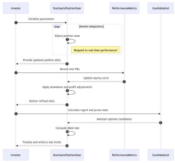
This brings us to what I have dubbed the Stochastic Position Sizer. A framework that treats position sizing not as a static formula but as a dynamic process. Indeed, translating the concept of adaptive, performance-contingent sizing into a functional algorithm requires defining specific rules and mechanisms.
The StochasticPositionSizer is designed to dynamically adjust position size based on the system's performance history, particularly its Profit and Loss and resulting equity curve. It is initialized with boundaries min_contracts, max_contracts and a starting size initial_contracts. Its adaptive behavior is governed by several key parameters:
drawdown_sensitivity: Controls how aggressively position size is reduced as the system enters or deepens a drawdown. Higher sensitivity leads to steeper reductions.profit_smoothing: Determines the influence of recent positive PnL on scaling up position size. A higher value allows recent profits to more readily increase size.recovery_rate: Specifies how quickly position size is increased towards theinitial_contractslevel when the system is showing signs of recovering from a drawdown—i.e., drawdown is shrinking.lookback_period: Defines the window size for calculating recent performance metrics, such as average PnL.
These parameters calibrate the sizer's response profile, allowing it to be more risk-averse during losses and more aggressive during profitable periods, according to the system designer's preference.
But before implementing it, let’s take a look of the mathematical background.
Mathematical foundations of adaptive sizing
The core of the StochasticPositionSizer's logic resides in how it mathematically adjusts the position size based on calculated performance metrics within its update method.
Drawdown-based size reduction
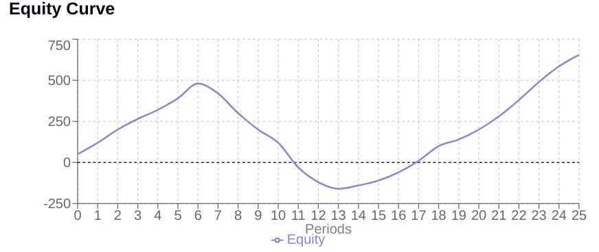
Drawdown (DD) is a critical metric representing the percentage decline from the peak equity reached so far. It is calculated as:
The absolute value in the denominator provides robustness, though for established positive equity curves, it simplifies to just the peak.
The size adjustment based on drawdown uses an exponential decay function:
Here, e is the base of the natural logarithm. This formula ensures a non-linear response: small drawdowns result in minor size reductions—factor close to 1—while larger drawdowns lead to increasingly aggressive reductions—factor decreasing rapidly towards 0. A higher drawdown_sensitivity makes this reduction curve steeper. This mechanism is fundamental for dynamic capital preservation during unfavorable periods.
Profit-based size increase
Positive recent performance encourages scaling up. The sizer looks at the average PnL over the lookback_period.
avg_pnl = sum(recent_pnl) / len(recent_pnl)This average PnL, relative to the equity scale (represented in the code by the sum of the equity curve for normalization), contributes to a growth_factor.
This factor influences how much of the remaining distance to the max_contracts is added to the current size:
distance_to_max = self.max_contracts - current_size
if distance_to_max > 0:
    contracts += distance_to_max * (1 - math.exp(-growth_factor)) * 0.1
The term 1−e−GrowthFactor increases towards 1 as GrowthFactor increases. The additional 0.1 multiplier in the code dampens this effect, ensuring that scaling up towards the maximum is gradual and smoothed, preventing over-leveraging based on short-term volatility spikes.
Recovery adjustment
When the system's drawdown percentage begins to decrease—prev_dd > self.current_drawdown—indicating a recovery phase, a specific adjustment is applied.
def _apply_recovery(self, contracts: float, improving: bool) -> float:
    if not improving:
        return contracts
    distance_to_initial = self.initial_contracts - contracts
    if distance_to_initial > 0: # Only if current size is below initial
        contracts += distance_to_initial * self.recovery_rate
    return contracts
If the system is improving and the current size is below the initial_contracts, a fraction or recovery_rate of the distance back towards the initial size is added. This provides a focused mechanism to help the position size rebound towards a baseline operating level once the system shows signs of emerging from a slump.
Algorithmic flow of the stochastic sizer
The update method integrates these calculations sequentially. Upon receiving a new PnL:
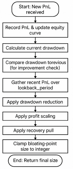
This flow ensures that risk-off—drawdown reduction—is a primary response, followed by risk-on—profit scaling—and recovery logic.
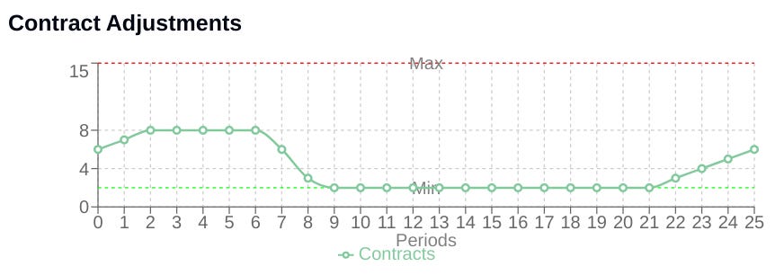
Besides, there are some granularity considerations. While the StochasticPositionSizer provides adaptive sizing, it calculates a floating-point target size and then rounds it to an integer. In many trading environments, position sizes are discrete integer units. This raises a question: is calculating a precise float necessary or potentially noisy? Constantly adjusting towards a theoretical continuous value before rounding might introduce small, frequent changes that aren't strictly necessary or could be sensitive to minor PnL variations. This highlights a potential area for refinement – managing the decision space to a discrete set of options.
Introducing abstraction via regret minimization
To address the granularity consideration and add a layer of stability, the AbstractedStochasticPositionSizer is introduced. This class maintains a limited set of candidate position sizes and, instead of simply rounding the calculated target size, selects the closest size from this curated list.
The selection and maintenance of this candidate list are managed using a form of regret minimization. After each PnL update, the system calculates the hypothetical PnL that would have been achieved if each candidate size s had been used instead of the actual sizet:
Where Size Usedt is self.current_contracts from the previous step in the code.
The system identifies the candidate size that yielded the highest hypothetical PnL for that step. The "regret" for every other candidate is the difference between the best hypothetical PnL and their own:
This regret accumulates for each candidate over a defined prune_interval.
Pruning of candidates
Periodically, after the prune_interval, the system prunes the candidate list based on the accumulated regret. Candidates are sorted by their total regret—lowest regret is best. Only the top target_range_size candidates with the least accumulated regret are retained. Their regret counters are reset to zero for the next interval.
# Snippet: Regret Update and Candidate Pruning
def _update_regrets(self, pnl: float):
    # Calculate hypothetical PnL for all candidates for this step
    hypo = {s: pnl * (s / (self.current_contracts or 1)) for s in self.candidate_sizes}
    best = max(hypo.values()) # Find the best outcome among candidates

    # Accumulate regret for those who weren't the best
    for s, val in hypo.items():
        self.regrets[s] += max(0, best - val)

def prune_candidates(self):
    # Sort candidates by total regret (lowest first) and keep the best
    best = sorted(self.regrets.items(), key=lambda x: x[1])[:self.target_range_size]
    self.candidate_sizes = [int(s) for s, _ in best]

    # Reset regret for the survivors
    self.regrets = {s: 0.0 for s in self.candidate_sizes}
This mechanism ensures that the candidate set remains focused on the sizes that have empirically performed well—relative to the other candidates—over recent history, filtering out those that consistently led to suboptimal hypothetical results.
Abstracted position sizer