


Table of contents:
Introduction.
The constraints of parametric models.
Traditional Random Forests vs Ordered Random Forests.
Implementing the basic architecture.
Mining market intelligence with order.
Test on Cboe’s SPX Options 2018‑04‑01 until today.
Before you begin, remember that you have an index with the newsletter content organized by clicking on “Read the newsletter index” in this image.

Introduction
So here’s the thing—financial markets are these complicated beasts where catching the right signal at the right time is everything. Yeah, we’ve got our continuous data staples like factor models, order book dynamics, and volatility metrics doing the heavy lifting. But let’s not kid ourselves: some of the juiciest predictive signals? They’re not neat numerical streams. They’re ordered buckets of information.
Take market sentiment indicators – you know, the whole spectrum from panic-selling bearish to meh to irrationally exuberant bullish. Earnings surprises? Always framed as trainwreck miss, near miss, on-target, modest beat, or blowout. Even price action gets chunked into clear tiers: violent selloffs, mild dips, sideways purgatory, hesitant rallies, full-throttle uptrends.
What makes these ordinal categories gold is their gradation – the fact that ‘mildly bullish’ sits between neutral and ‘raging bull’ isn’t just trivia, it’s structural alpha. But here’s where things get tricky: most ML models either treat them like random labels —ignoring the order entirely—or force them into some linear regression framework —pretending the steps between categories are uniform. Both approaches leave money on the table. One strips out hierarchy, the other imposes false mathematical relationships. It’s this weird paradox in quant work – we’ve got all these beautifully ordered signals, but keep analyzing them with tools that either flatten or contort their actual shape.
As the statistician George Box famously stated:
"Essentially, all models are wrong, but some are useful." Our challenge is to find the model most useful for capturing the essential ordered structure of financial signals, rather than distorting it.
The constraints of parametric models
For decades, quants and traders dealing with ordered outcomes relied heavily on parametric models, primarily ordered logit and ordered probit. These models postulate an underlying latent continuous variable related to the predictors through a linear function and thresholds that map the latent variable to the observed ordered categories. While mathematically elegant under their specified conditions, their application to the chaotic, high-dimensional, and non-linear world of financial markets is fraught with peril.
The key limitations include:
They assume a linear relationship between the predictors and the latent variable. Market dynamics, however, are notoriously non-linear.
Ordered logit models, for instance, often assume that the effect of any predictor is the same across all cumulative splits—i.e., the odds ratio between adjacent categories is constant. This parallel lines assumption rarely holds true in complex systems like financial markets where feature effects can vary dramatically depending on the market state or level of the outcome.
Ordered probit assumes the error term follows a standard normal distribution, while ordered logit assumes a logistic distribution. Financial data error distributions are often heavy-tailed and deviate significantly from these standard assumptions.
These models struggle to naturally capture complex interaction effects between predictors without explicit, often manual, interaction term specification.
Their performance can degrade in datasets with a large number of correlated or irrelevant features, common in quantitative trading.
In algorithmic trading, predictive accuracy is not an abstract metric; it translates directly into profitability and risk management effectiveness. The restrictive assumptions of parametric models represent a tangible drag on potential trading edge, limiting the ability to fully exploit the subtle, non-linear relationships driving ordered market states.

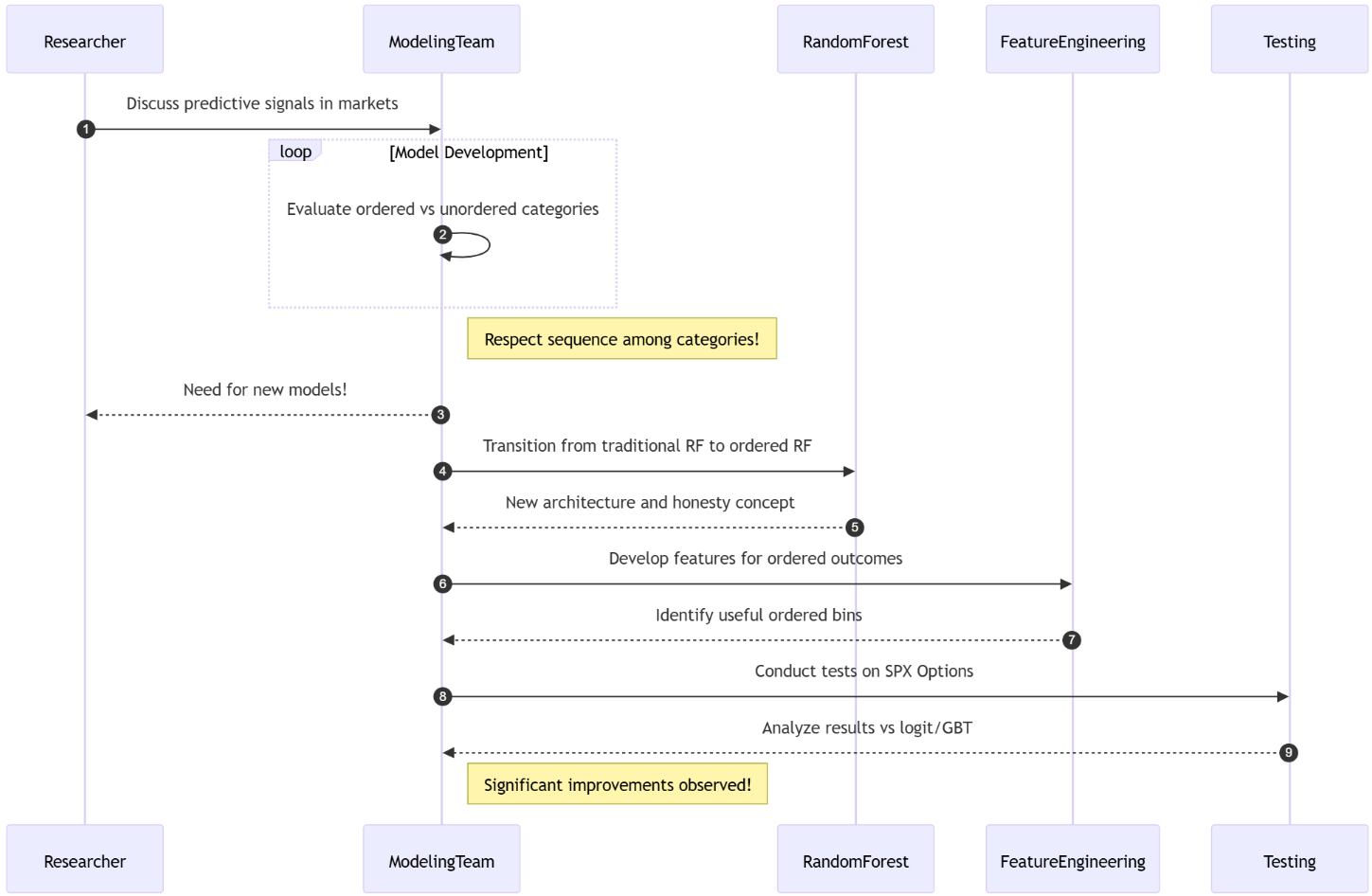
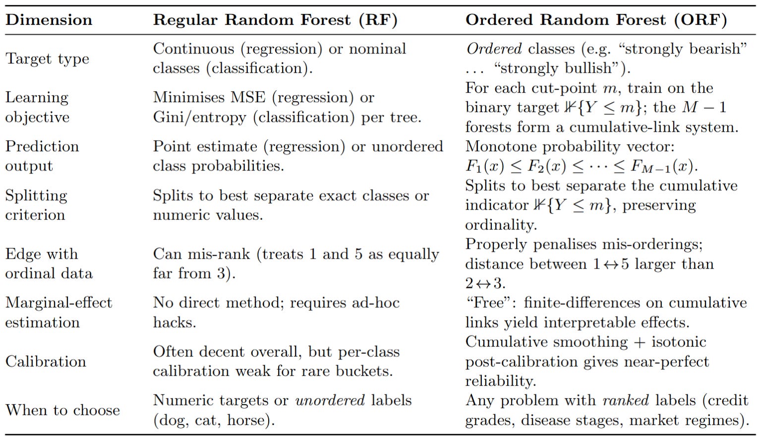
Traditional Random Forests vs Ordered Random Forests
The truth is, there aren't many algorithms in the literature that model ordered events—pretty suitable for news trading. So let's look at a classic: Ordered Random Forests. Less random and more ordered. There are substantial differences when choosing which type of model to use in trading. It's common to see quants using the traditional random forest. But what advantages are there in choosing one over the other?
You can see it in this summary table:
The advent of the Ordered Random Forest, primarily formalized by Lechner and Okasa (2019)—I'll leave it a little further down for you—marks a significant paradigm shift. It liberates the modeling of ordered categorical outcomes from the confines of rigid parametric assumptions by adopting the flexible, non-linear, and ensemble-based power of random forests. The core innovation lies in reframing the ordered classification problem into a series of binary classification tasks related to cumulative probabilities.
Traditional random forests for regression estimate:
Where Tb(x) represents individual tree predictions and B is the number of trees. You can read more about RFs here:

For ordered categorical outcomes with M categories, we need a fundamentally different approach. Instead of directly predicting the category m, the ORF models the probability of being in category m or any category below it. For an outcome Yi with M ordered categories {c1,c2,...,cM} and a vector of predictors Xi, the ORF estimates the cumulative probabilities:
This is achieved by training M−1 separate random forests. The m-th forest is trained to predict the binary outcome I(Yii≤cm ), where I(⋅) is the indicator function.
Once these cumulative probabilities are estimated, the probability of being in a specific category cm is derived:
with the boundary conditions:
This methodology retains the explicit ordering of the categories while benefiting from the advantages of random forests:
Non-parametric flexibility.
Automatic interaction capture.
Robustness to high-dimensionality.
Consistent probability estimation.
Principled marginal effects.
The Ordered Forest thus represents a fundamental step forward, offering algorithmic traders a powerful tool specifically designed to leverage the information embedded in ordered categorical market signals.
If you want to go deeper in this type of model, check this:

Implementing the basic architecture
Let's break it down and consider the improvements over the traditional implementation. I want to emphasize once again the importance of using categorical data, such as events, for this algorithm. Here the pseudocode to implement:
Okay! So the base model would be as follows:
import numpy as np
import pandas as pd
from sklearn.ensemble import RandomForestRegressor
import itertools # Needed for grid search

class OrderedForest:
    def __init__(self, n_estimators=1000, min_samples_leaf=5,
                 max_features='sqrt', random_state=42, **kwargs):
        self.n_estimators = n_estimators
        self.min_samples_leaf = min_samples_leaf
        self.max_features = max_features
        self.random_state = random_state
        self.forests = []
        self.classes_ = None
        # Store additional RF parameters
        self.rf_params = kwargs

    def fit(self, X, y):
        # Ensure X is a numpy array for consistent indexing
        X = np.asarray(X)
        y = np.asarray(y)

        # Store unique classes in sorted order
        self.classes_ = np.sort(np.unique(y))
        n_classes = len(self.classes_)

        if n_classes < 2:
            raise ValueError("Input data must contain at least two unique classes.")

        # For each cutpoint, build a random forest for cumulative probability
        # There are M-1 cutpoints for M classes
        for m in range(n_classes - 1):
            # Create binary indicator: 1 if y <= class_m, 0 otherwise
            # Using <= self.classes_[m] correctly defines the cumulative target
            y_binary = (y <= self.classes_[m]).astype(int)

            # Train random forest for this cutpoint
            # Use the stored rf_params
            forest = RandomForestRegressor(
                n_estimators=self.n_estimators,
                min_samples_leaf=self.min_samples_leaf,
                max_features=self.max_features,
                random_state=self.random_state + m, # Vary state for diversity
                **self.rf_params # Pass additional params
            )
            forest.fit(X, y_binary)
            self.forests.append(forest)

        return self

    def predict_proba(self, X):
        # Ensure X is a numpy array
        X = np.asarray(X)
        n_samples = X.shape[0]
        n_classes = len(self.classes_)

        if not self.forests:
             raise RuntimeError("Model has not been fitted yet.")

        # Get cumulative probabilities from each forest
        # Initialize with zeros for the P(Y <= c_0) = 0 boundary
        cum_probas = np.zeros((n_samples, n_classes))

        # The first column is P(Y <= c_0) = 0
        # The last column will conceptually be P(Y <= c_M) = 1, handled in differencing

        for m in range(n_classes - 1):
            # Ensure predictions are clipped to [0, 1] range
            cum_probas[:, m+1] = np.clip(self.forests[m].predict(X), 0, 1)

        # Calculate class probabilities from cumulative probabilities
        # probas[:, m] = P(Y <= c_m) - P(Y <= c_{m-1})
        probas = np.diff(cum_probas, axis=1)

        # Ensure all probabilities are non-negative due to potential small prediction errors
        probas = np.maximum(0, probas)

        # Normalize to ensure rows sum to 1, addressing potential floating point issues
        # Add a small epsilon to avoid division by zero if a row sums to zero (shouldn't happen in theory)
        row_sums = probas.sum(axis=1)
        probas = probas / (row_sums[:, np.newaxis] + 1e-9)

        return probas

    def predict(self, X):
        probas = self.predict_proba(X)
        # Return the class label corresponding to the highest probability
        return self.classes_[np.argmax(probas, axis=1)]

    # Add a method to get cumulative probabilities
    def predict_cumulative_proba(self, X):
         X = np.asarray(X)
         n_samples = X.shape[0]
         n_classes = len(self.classes_)
         cum_probas = np.zeros((n_samples, n_classes + 1)) # Include boundaries

         if not self.forests:
              raise RuntimeError("Model has not been fitted yet.")

         # P(Y <= c_0) = 0 is the first column (cum_probas[:, 0])
         for m in range(n_classes - 1):
             cum_probas[:, m+1] = np.clip(self.forests[m].predict(X), 0, 1)
         # P(Y <= c_M) = 1 is the last column (cum_probas[:, -1])
         cum_probas[:, -1] = 1.0

         return cum_probas
A critical concept in the original orf implementation—though not strictly necessary for a basic predictive model like the one above, it's vital for valid inference like marginal effects—is honesty:
An honest forest splits the data into two parts: one for determining the tree structure—split points—and another for estimating the values in the leaf nodes.
For regression forests predicting probabilities, this means the data used to decide splits should be distinct from the data used to calculate the average binary target value in the leaves. This helps prevent overfitting and ensures consistent estimation, particularly for prediction-weighted statistics like marginal effects. Implementing honesty would involve a more complex fit method that handles this internal data splitting for each tree.

Mining market intelligence
The predictive power of an Ordered Forest is intrinsically linked to the quality and relevance of its input features. For ordered categorical outcomes in trading, features that capture the degree or intensity of a market condition are particularly valuable. These features often have inherent thresholds or levels that align naturally with ordered categories.
Beyond the examples provided, consider:
Categorizing volatility—e.g., VIX index levels for equity markets—into low, medium, high, extreme.
Classifying assets or time periods based on trading volume or bid-ask spread into highly liquid, moderately liquid, low liquidity.
Quantifying the surprise component of economic data releases—e.g., CPI, NF— into significant negative surprise, slight negative surprise, in-line, slight positive surprise, significant positive surprise.
Aggregating analyst ratings into strong sell, sell, hold, buy, strong buy.
The key takeaway is that feature engineering for ORF should focus on creating variables that naturally stratify market conditions into ordered levels, supplementing these with relevant continuous features.
The output you get with this type of data is like this one:
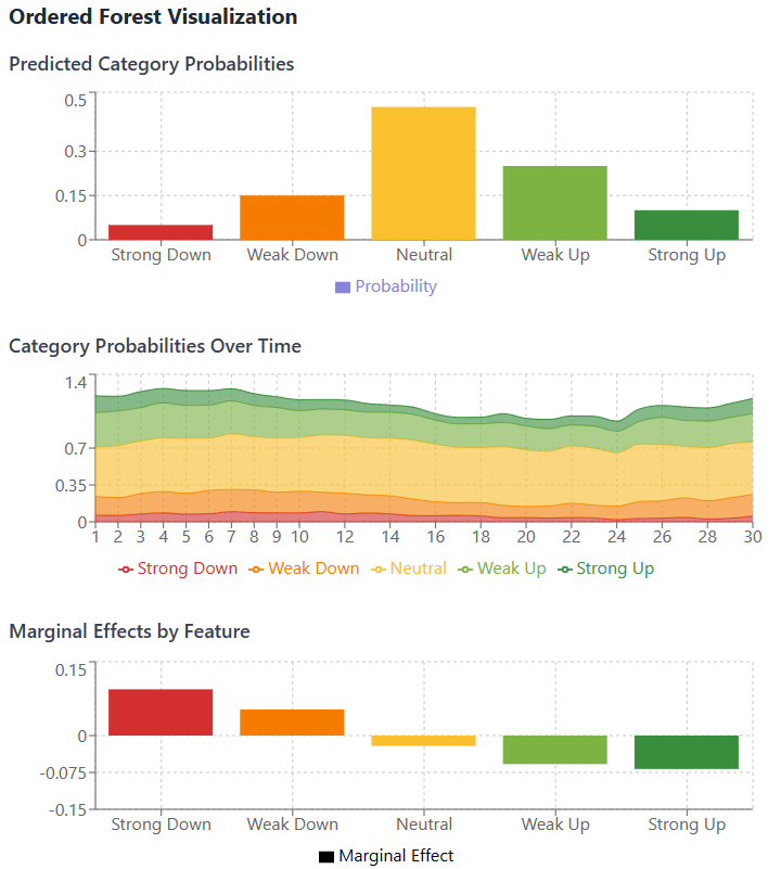
Besides, one of the most valuable diagnostic tools provided by the Ordered Forest is the ability to estimate marginal effects as we see in the picture above. Unlike parametric models where marginal effects are derived from the model's functional form and distribution assumptions, ORF estimates them non-parametrically by evaluating the change in the predicted probability distribution when a feature's value is perturbed, holding other features constant.
The marginal effect of a continuous feature Xk on the probability of outcome category cm at a specific point x in the feature space is approximated using a finite difference:
where h is a small perturbation, and X-k denotes all features except Xk. For categorical features, the marginal effect is the difference in predicted probabilities when the feature changes from one category to another.
For algorithmic traders, these marginal effects are not just theoretical constructs; they are actionable insights:
Quantify how much a change in a predictor impacts the probability of future price movements → signal strenght and direction.
Pinpoint which features have the most significant influence on the ordered outcome probabilities in different market contexts → identifying key drivers.
Marginal effects can vary depending on the current feature values, revealing non-linear relationships that parametric models miss.
Marginal effect can be implemented as: