

[WITH CODE] Model: Robust threshold estimation
Can you trust your thresholds? Test Jackknife‐after‐bootstrap

Table of contents:
Introduction.
Identification of potential pitfalls.
Facing data challenges.
The classic Jackknife.
Constructing robust intervals with JackKnife++.
Jackknife‐after‐bootstrap.
Understanding the bootstrap stage.
Integrating the Jackknife.
Overcoming obstacles.
Before you begin, remember that you have an index with the newsletter content organized by clicking on “Read full story” in this image.

Introduction
In quantitative analysis a robust threshold estimate is vital. Picture having to decide when to trigger a trade, or when a process reaches a critical safety limit, based solely on data that is inherently noisy. As a quant, I often find that the task is not just to compute a value but to assign a degree of confidence to it.
Consider a threshold estimator defined as
where Q(p) denotes the pth quantile of the observed data. The use of quantiles, rather than moments like the mean, naturally brings in robustness against outliers. However, even with quantile-based estimation, finite samples rarely represent the true underlying distribution perfectly. Bias may creep in, variability can be underestimated, and overconfident predictions might follow—all of which could lead to significant misjudgments when these estimators are deployed in high-stakes environments.
The initial dilemma is clear: how can one compute the threshold T from financial data and simultaneously account for uncertainties to produce reliable intervals for decision-making? A naive approach might compute T directly, but without further analysis, the risks remain hidden.
Identification of potential pitfalls
Every robust estimation problem comes with its share of risks. In designing a reliable estimator for T, I identified the following principal hazards:
Risk of bias: Because the estimator T is based on the 70th and 30th quantiles, its finite-sample values may differ from the true quantiles of the underlying distribution. This can lead to a systematic bias—an error that does not diminish with more data if not properly corrected.
Risk of variability underestimation: A point estimate is only as good as our understanding of its variability. If we underestimate the spread or the standard error of T, we may produce confidence intervals that are too tight. In practice, this overconfidence can lead to undesirable decisions, as small fluctuations might push the system into an unstable regime.
Risk of outliers: Although quantiles are intrinsically robust, unusual observations or extreme values in small samples may still disturb the estimated values. Their influence could be disproportionate if the sample density in the quantile regions is low.
Understanding these pitfalls is essential for selecting the right methods to address them. Ultimately, the goal is to develop resampling methodologies that mitigate these issues and yield robust, trustworthy threshold estimates.
A few years back, during routine simulation studies, it became starkly apparent that our initial, direct computations of T were too optimistic. Confidence intervals derived from standard asymptotic approximations were far too narrow. In one notable simulation, a single outlier skewed the quantile estimates, and the resulting threshold failed to capture the underlying variability of the process. This event was a wake-up call: relying solely on direct estimation techniques, without addressing bias and uncertainty properly, could result in decisions based on overconfident, misleading statistics.
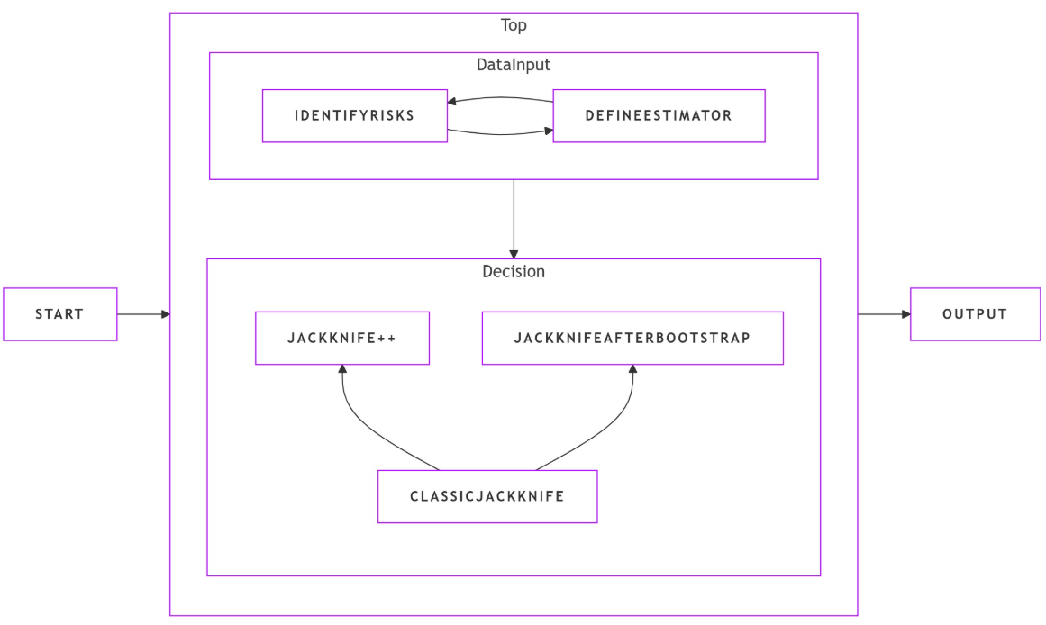
That moment of clarity set me on a path to explore advanced resampling methods. I turned my attention to three key methodologies:
The classic Jackknife: A straightforward method to assess bias and estimate variability by systematically omitting one data point at a time.
Jackknife++: An evolution of the classic method that constructs robust prediction intervals through analysis of leave-one-out residuals.
Jackknife‐after‐bootstrap: A hybrid approach that blends bootstrap replication with jackknife correction to handle particularly challenging data scenarios.
If you want a little more detail you can find it here:
Facing data challenges
Imagine being at the helm of a vessel navigating through stormy seas. The ship represents our threshold estimator T and the turbulent waves symbolize the inevitable noise and uncertainty in real-world datasets. As a quant, the mission is to steer this ship reliably, regardless of how rough the data's waters become.
The chief challenge lies in answering two critical questions: Is T unbiased? And how accurately can we assess its uncertainty? Traditional statistical methods based on central limit theorem approximations often break down when confronted with finite data and unexpected deviations. Instead, we must adopt methods that iteratively resample our data—examining it from every possible angle—to gauge the true stability and variability of T.
The challenge then is to implement resampling techniques that address both bias correction and uncertainty quantification, ensuring that our computed threshold does not mislead by appearing deceptively precise.

The classic Jackknife
The classic jackknife is a method I first encountered as a simple but powerful tool to assess the influence of individual data points on an estimator. For a sample {x1,x2,…,xn}, we compute the full-sample estimate Tfull=T(x1,x2,…,xn) and then calculate leave-one-out estimates
for each i. From these nnn recalculations, a family of estimates emerges that mirrors the variability inherent in the data.
The bias-corrected jackknife estimator is defined as
with
The accompanying standard error is given by
This method is much like a detective removing one suspect at a time to determine each one's influence on the final verdict. It tells you precisely how sensitive the estimator is to each piece of data.
Okay! Let’s implement the classic Jackknife to calculate the treshold T and its bias-corrected version!
import numpy as np
import matplotlib.pyplot as plt

def threshold_estimator(serie):
    """
    Calculates the threshold as the average of the 70th and 30th quantiles.
    """
    return (np.quantile(serie, 0.7) + np.quantile(serie, 0.3)) / 2

def jackknife_threshold(serie):
    """
    Applies the classic jackknife method to estimate the threshold and its standard error.

    Parameters:
        serie : array-like
            The input data vector.

    Returns:
        T_jack : float
            The bias-corrected jackknife estimate.
        std_error : float
            The jackknife estimated standard error.
        jackknife_estimates : ndarray
            Array of leave-one-out estimates.
    """
    n = len(serie)
    jackknife_estimates = np.empty(n)

    # Perform leave-one-out resampling
    for i in range(n):
        sample_i = np.delete(serie, i)
        jackknife_estimates[i] = threshold_estimator(sample_i)

    T_full = threshold_estimator(serie)
    T_bar = np.mean(jackknife_estimates)
    T_jack = n * T_full - (n - 1) * T_bar
    std_error = np.sqrt(((n - 1) / n) * np.sum((jackknife_estimates - T_bar) ** 2))

    return T_jack, std_error, jackknife_estimates

# Simulated data for demonstration
np.random.seed(42)
data_large = np.random.randn(1000)

T_full = threshold_estimator(data_large)
T_jack, se_jack, jk_estimates = jackknife_threshold(data_large)

print("Classic Jackknife results:")
print(f"Full-sample estimate: {T_full:.4f}")
print(f"Jackknife bias-corrected estimate: {T_jack:.4f}")
print(f"Jackknife standard error: {se_jack:.4f}")
The output is:
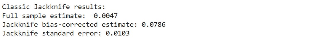
Pretty far from the full sample bias-corrected estimate, right?!
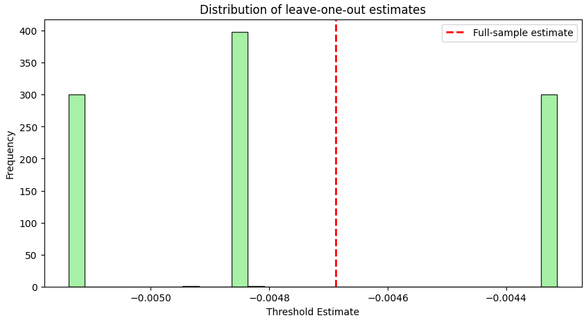
In the resulting histogram, the red dashed line indicates the full-sample estimate Tfull. The spread of the leave-one-out estimates reveals the inherent variability of our data—and thus the uncertainty in our threshold estimation.
Constructing robust intervals with JackKnife++
Even though the classic jackknife does an admirable job of bias correction and variance estimation, it does not provide a direct path to constructing full confidence or prediction intervals. To address this, I turned to Jackknife++, a method that enhances the classic approach by focusing on the residual differences between the full-sample and leave-one-out estimates.
For each observation i, define the residual
Next, by computing the (1−α) quantile of the residuals—for example, the 95th percentile when α=0.05—denoted q1−α, we define the prediction interval as
This approach is analogous to casting a net around the estimator that adapts to the observed variability in the data. Instead of settling for a single error estimate, Jackknife++ uses the distribution of residuals to ensure that the entire range of potential fluctuations is captured.
Let’s implement the method!
def jackknife_plus_threshold(serie, alpha=0.05):
    """
    Applies the Jackknife++ method to construct a prediction/confidence interval for the threshold estimator.

    Parameters:
        serie : array-like
            The data vector.
        alpha : float, significance level (default 0.05 for a 95% interval).

    Returns:
        T_full : float
            The full-sample threshold estimate.
        lower_bound : float
            The lower bound of the prediction interval.
        upper_bound : float
            The upper bound of the prediction interval.
        jackknife_estimates : ndarray
            Array of leave-one-out estimates.
        residuals : ndarray
            Array of absolute residuals between T_full and leave-one-out estimates.
    """
    n = len(serie)
    jackknife_estimates = np.empty(n)

    # Compute leave-one-out estimates
    for i in range(n):
        sample_i = np.delete(serie, i)
        jackknife_estimates[i] = threshold_estimator(sample_i)

    T_full = threshold_estimator(serie)
    residuals = np.abs(jackknife_estimates - T_full)
    quantile = np.quantile(residuals, 1 - alpha)

    lower_bound = T_full - quantile
    upper_bound = T_full + quantile

    return T_full, lower_bound, upper_bound, jackknife_estimates, residuals

T_full_plus, lower_bound, upper_bound, jk_est_plus, residuals = jackknife_plus_threshold(data_large, alpha=0.05)

print("Jackknife++ Interval:")
print(f"Full-sample estimate: {T_full_plus:.4f}")
print(f"95% Prediction Interval: [{lower_bound:.4f}, {upper_bound:.4f}]")
If you check the output you will see something like:
And if you plot it:
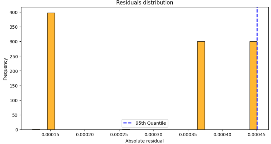
In this case, the blue dashed line in the residual histogram indicates the 95th percentile of the residuals. This value determines the width of the prediction interval, ensuring that nearly all of the leave-one-out estimates fall within the specified bounds.
Jackknife‐after‐bootstrap