[WITH CODE] Model: Very Fast Decision Rules
Do statistical guarantees hold in unpredictable markets?

Table of contents:
Introduction.
Risks associated with VFDR.
Data stream acquisition and management.
Rule induction and generation in VFDR.
The hoeffding bound and statistical guarantees.
Data simulation and VFDR integration.
Before you begin, remember that you have an index with the newsletter content organized by clicking on “Read full story” in this image.

Introduction
Sometimes decisions must be made at an unprecedented pace, with prices fluctuating by fractions of a second. Traditional static models can be too slow or cumbersome to adapt to market dynamics. Herein lies the initial dilemma:
how do we construct a framework that not only processes data streams quickly but also adapts its decision rules on the fly, ensuring both speed and accuracy under pressure?
The concept of Very Fast Decision Rules was born from this need—its promise lies in rapidly generating decision rules by dynamically processing streaming data. VFDR is designed to operate under conditions where the data are continuously arriving at high velocities, as seen in modern trading platforms. The algorithm aims to continuously learn and adjust to the trading environment, exploiting minute discrepancies and fleeting arbitrage opportunities before they vanish.
Risks associated with VFDR
While VFDR heralds a new era in adaptive decision-making, it also introduces a set of unique risks:
If the data is not properly curated and transformed, the probability of obtaining overfitting rules is quite high.
VFDR relies on probabilistic guarantees—such as those provided by the Hoeffding bound—to make early decisions. Misestimating these bounds can lead to premature rule acceptance or rejection.
The data streams can be erratic or influenced by external market events. Robust preprocessing and noise filtering become critical to prevent erroneous decisions.
Knowing that, imagine a sudden crash—a moment when market prices plummet superfast due to a cascade of algorithmic triggers. In such a crisis, traditional methods crumble, and VFDR’s potential to adapt and respond rapidly comes into sharp focus.
It is this pivotal event—a market anomaly triggered by the interplay of high-speed trading algorithms—that underscores the necessity for systems capable of ultra-rapid decision-making with strong theoretical guarantees. This moment becomes the driving force behind VFDR research and its prospective application in algorithmic trading frameworks.
You can go deeper in this algorithm by checking this:
We are going to implement a simplified version that includes some changes.
Data stream acquisition and management
Algorithmic trading operates on a relentless torrent of data—each tick, trade, and quote contributes to a vast, ever-flowing river of information. In this environment, VFDR must learn and update its decision rules from a continuous data stream. The challenge begins at the very source: how do we efficiently manage and preprocess this information to feed our algorithm without succumbing to the sheer volume and variability?
Data stream management involves:
Real-Time preprocessing: Filtering out noise and spurious events while preserving relevant market signals.
Incremental updates: Leveraging online learning techniques to update decision rules without having to retrain models from scratch.
Memory and computational constraints: Ensuring that the algorithm runs efficiently within available hardware limitations.
Let us denote the incoming data stream as {x1,x2,…,xt}, where each xi represents a feature vector extracted from market data at time i. The goal is to construct a sequence of decision rules Rt such that the predictive performance P(Rt) is maximized subject to a computation time constraint Tcomp.
In mathematical terms, we can express the VFDR update strategy as:
where ΔRt represents the incremental update based on the new data point xt+1 and Tmax is the maximum allowed processing time per update.
Let’s see an example that simulates real-time data ingestion for our VFDR.
import numpy as np
import time

def simulate_market_data(n_points=1000):
    """Simulate market data as a stream."""
    # For illustrative purposes: simulate price changes following a random walk
    prices = np.cumsum(np.random.randn(n_points)) + 100
    return prices

def preprocess_data(data_point):
    """Simple preprocessing: here, you might filter noise, compute returns, etc."""
    # In a real-world scenario, consider using smoothing techniques or anomaly detection
    return np.clip(data_point, 0, np.inf)

# Simulate a data stream
data_stream = simulate_market_data(1000)
processed_stream = [preprocess_data(point) for point in data_stream]

# Simulate incremental processing with VFDR (placeholder for decision rule updates)
for idx, data_point in enumerate(processed_stream):
    # Simulate processing delay (ideally sub-millisecond in live trading)
    time.sleep(0.001)
    # Update VFDR model here (not implemented in this simple simulation)
    if idx % 100 == 0:
        print(f"Processed {idx} data points")
This represents a foundational step in handling market data—a prerequisite for any VFDR-based system. Think that this is a toy example, in an actual implementation, the preprocessing function would require more customization for your data and features.
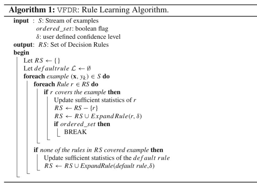
Rule induction and generation in VFDR
At the heart of VFDR lies the ability to construct decision rules rapidly. These rules determine whether to buy, hold, or sell based on specific patterns in the data. The uniqueness of VFDR is its capability to evolve rules in near-real-time by considering both the current market conditions and historical trends.
Imagine a discretionary trader making split-second decisions in a bustling trading floor; VFDR is designed to emulate that intuition by inductively learning rules from the continuous influx of market signals. The underlying challenge is to strike the right balance between decisiveness and prudence.
The process can be broken down into:
Feature Extraction: Selecting pertinent features that capture the essence of market behavior. Examples include price volatility, moving averages, and momentum indicators.
Rule Hypothesis Testing: Given a potential decision rule—e.g., “if the short-term moving average exceeds the long-term moving average, then buy”—the VFDR framework evaluates its performance incrementally.
Adaptive Updating: As new data arrive, the algorithm revises the rule parameters to reflect the evolving market landscape.
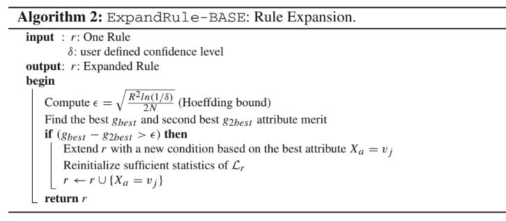
To get a clearer idea this pseudo code may be useful:
Consider a rule R represented as a logical expression over market features. The quality Q(R) of a rule can be quantified using a performance metric such as the Gini impurity or information gain. For a binary classification task—e.g., buy or not buy—the information gain IG is defined as:
where:
H(Y) is the entropy of the output variable—trading decision.
N is the total number of instances.
Nv is the number of instances for a given rule value v.
H(Y|R=v) is the conditional entropy of Y given the rule R.
The VFDR algorithm continually computes these quantities in an online manner to decide when a decision rule is statistically significant enough to be deployed in real time.

We can implement the computation of information gain for a simple rule with this:
import numpy as np

def entropy(probabilities):
    """Compute entropy given a list of probabilities."""
    return -np.sum([p * np.log2(p) for p in probabilities if p > 0])

def compute_information_gain(rule_outcomes, total_outcomes):
    """
    Compute the information gain of a rule.
    rule_outcomes: dictionary with keys as rule value and values as count of occurrences
    total_outcomes: dictionary with overall outcome counts
    """
    total_samples = sum(total_outcomes.values())
    overall_entropy = entropy([count / total_samples for count in total_outcomes.values()])

    weighted_entropy = 0
    for rule_value, count in rule_outcomes.items():
        subset_total = count
        subset_entropy = entropy([count / subset_total for count in rule_outcomes.values()])
        weighted_entropy += (subset_total / total_samples) * subset_entropy

    return overall_entropy - weighted_entropy

# Example usage:
total_outcomes = {'buy': 500, 'hold': 300, 'sell': 200}
rule_outcomes = {'buy': 300, 'hold': 100, 'sell': 100}
ig = compute_information_gain(rule_outcomes, total_outcomes)
print(f"Information Gain for the rule is: {ig:.4f}")
This provides a simplified glimpse into one of the core components of VFDR: the evaluation and selection of decision rules based on their information gain.
The hoeffding bound and statistical guarantees
One of the key theoretical pillars of VFDR is the Hoeffding bound. This statistical tool provides an upper bound on the difference between the true mean of a random variable and its estimated mean from finite samples. In the context of VFDR, the Hoeffding bound is used to determine the number of observations needed before confidently adopting a decision rule.
The Hoeffding bound states that, for a random variable X bounded by a≤X≤b, after n independent observations, with probability 1−δ the true mean μ is no more than:
In VFDR, let hat μ denote the empirical performance measure—e.g., accuracy or information gain—of a decision rule after nnn samples. The algorithm uses the Hoeffding bound to check whether the difference between the best candidate rule and the second-best candidate is statistically significant. When:
the algorithm can safely commit to R1 as the better decision rule.
This mathematical guarantee allows VFDR to make decisions quickly without requiring the evaluation of every possible rule exhaustively—a critical requirement if you want to face low latency setups.
Okay, let’s visualize how the Hoeffding bound ϵ\epsilonϵ decreases as the number of observations nnn increases.
import matplotlib.pyplot as plt
import numpy as np

def hoeffding_bound(n, a=0, b=1, delta=0.05):
    return np.sqrt(((b - a) ** 2 * np.log(1 / delta)) / (2 * n))

n_values = np.arange(1, 1000, 1)
epsilon_values = [hoeffding_bound(n) for n in n_values]
For this we get:
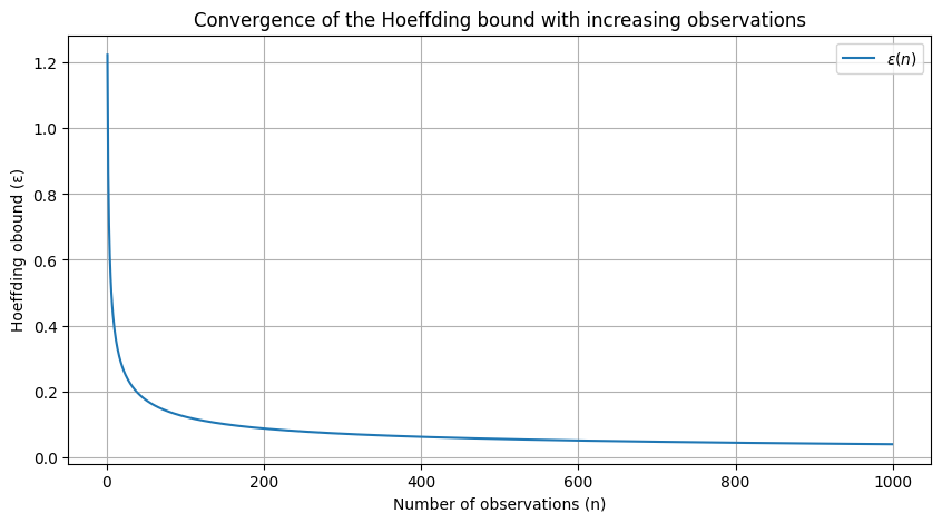
This plot illustrates that as the number of observations increases, the Hoeffding bound ϵ decreases, thereby reducing the uncertainty associated with rule performance estimates.
The significance of the Hoeffding bound in VFDR cannot be overstated. It is the mathematical linchpin that enables quick decision making by offering a probabilistic guarantee on the performance of a rule. By setting a confidence threshold δ, traders can calibrate the VFDR system to the desired level of risk tolerance. The interplay between n, δ, and the bound ϵ becomes a trade-off between precision and caution—and also speed-acuracy.
Once again you can take a look at the above mentioned through: