

[WITH CODE] Market Making: Avellaneda–Stoikov model
Can you manage inventory—or is it managing you? Optimizing every microsecond of exposure

Table of contens:
Introduction.
Limitations from Avellaneda-Stoikov framework.
Algorithmic architecture.
Optimal quotes.
Inventory management dynamics.
Avellaneda-Stoikov Implementation.
Model improvements and lines of research.
Before you begin, remember that you have an index with the newsletter content organized by clicking on “Read full story” in this image.

Introduction
Alright, let’s break this down like we’re chatting over coffee. You know how market making feels? It’s like playing high-speed whack-a-mole in a casino where the moles are microseconds, and the casino’s on fire. Your job? Be the guy who’s always shouting “I’ll buy!” and “I’ll sell!” at the same time, pocketing the spread—that tiny gap between bid and ask. Sounds simple, right? Nah. It’s a brutal game of razor-thin margins and oh crap moments.
Here’s the kicker: you want that spread as wide as possible to cash in, but go too wide and nobody trades with you. You’re just yelling into the void. Too tight? Congrats, you’re now the exit liquidity for every algo shark with a faster connection. And that’s just the warm-up.
Let’s talk risks. First up, directional risk. Imagine you buy 10,000 shares of Stock X at 50, planning to flip them quick at 50.05. But then earnings drop, and suddenly it’s tanking to $48. Now you’re stuck holding a bag of regret. Classic. Then there’s inventory risk—you’re supposed to stay neutral, like a Switzerland of liquidity. But sometimes you end up long or short, sweating bullets because every tick feels like a heart attack. It’s like juggling chainsaws while balancing on a yoga ball.
And don’t get me started on adverse selection. You post a juicy ask price, thinking you’re slick, but some HFT fratboy front-runs you, sniffing out a market move you didn’t see. Now your safe quote is a liability. Oh, and volatility? When markets go haywire, your models start crying.
So how do you survive? Back in the day, it was all gut instinct and superstition—like trading on a horoscope. Then Avellaneda-Stoikov dropped in 2008 and changed the game. Finally, math to the rescue! They turned market making into an optimization problem: balance inventory risk against spread profit, using stochastic calculus.
But Avellaneda-Stoikov has quite a few mistakes. In fact, I started discussing this topic with a colleague following a request from a subscriber. And today I'm bringing you some of the notes. I don't want to be too hard on the math, but there are indices everywhere these days.
Limitations from Avellaneda-Stoikov framework
Think of the basic Avellaneda–Stoikov model as a beautifully crafted blueprint for a theoretical airplane. It shows the perfect aerodynamic shape, the ideal engine size. But to actually fly it, you need to contend with real-world wind gusts, turbulence, fuel impurities, and the fact that your passengers aren't dimensionless points. These limitations are the real-world factors that challenge the ideal flight plan.
Let's break down these friction points:
Unrealistic model assumptions:
The model assumes random, independent order fills. In reality, orders cluster and influence each other, making fill probabilities less predictable than the model assumes.
Prices are modeled as smoothly random with fixed volatility. But markets have volatile periods that jump and cluster, leading to inaccurate risk estimates and potentially mistimed quotes.
The model assumes your trading doesn't affect the market price—But if you can afford to do market making, you will probably affect the price.. Large trades actually move the market against you, a crucial cost the basic model ignores.
Parameter calibration challenges:
Pinpointing how order flow responds to your quote distance is complex, requiring analysis of noisy, high-speed data, and these parameters aren't stable.
The model assumes your tolerance for risk is constant. This can lead to suboptimal choices; ideal strategies might require adapting risk levels.
The model uses a basic curve for how fill probability drops with distance. Real market depth is more complex, making the model's spread calculations less precise.
Microstructure limitations:
Markets have minimum price steps and orders are filled in sequence at each price. The continuous model ignores these, missing key factors affecting execution probability and speed.
The model overlooks the cost of trading, which eats into profits and makes theoretical spreads appear more lucrative than they are.
The model assumes instantaneous order placement. Delays expose quotes to informed traders who can exploit outdated prices before you can react.
You can go deeper by reviewing this paper from Avellaneda & Stooikov (2006):

In short, it's not a model to use for the average person, I want to make this clear. But at the same time, I would like to have a chat with you to learn about your lines of work in this dynamic inventory control. Because at the end of the day, trading is about these two things:
Pricing.
Inventory.


Algorithmic architecture
At the heart of the Avellaneda–Stoikov model beats the concept of the reservation price r. This is not simply the observed market mid-price S, but rather the market maker's own, adjusted internal valuation of the asset. Think of it as your personal equilibrium point, a reference from which you calculate your willingness to buy or sell. What adjusts this internal compass? Your inventory q.
The formula is elegantly simple yet profoundly insightful:
Let's unpack this. The current market mid-price is the starting point. The subsequent term, −qγσ2(T−t), is the inventory risk adjustment.
q: Your current inventory. If q>0, you are long; if q<0, you are short.
γ: Your risk aversion parameter. This is your personal knob for how much pain inventory imbalance causes you. A higher γ means you really dislike holding inventory.
σ2: The volatility of the asset price. Higher volatility means the price can swing more wildly, making your current inventory position riskier.
(T−t): The time remaining until the end of your trading horizon. As time runs out, the urgency to flatten your position increases, making inventory risk more potent.
The negative sign in front of the adjustment term is crucial. If you are long, this term is negative, pushing your reservation price down. Why? Because you want to sell your excess inventory. By lowering your internal perceived value, you signal your willingness to sell at a price lower than the current market mid-point, incentivizing buyers. Conversely, if you are short, the term −qγσ2(T−t) becomes positive—negative times negative—pushing your reservation price up. You want to buy back your short position. A higher reservation price indicates a willingness to buy at a price higher than the market mid-point, attracting sellers.
This dynamic adjustment of the reservation price based on inventory is the model's core mechanism for steering you back towards a neutral inventory state, acting like a self-correcting feedback loop.
Optimal quotes
Another important point here is the optimal quotes. Once the reservation price is established, the optimal bid and ask quotes are derived. These quotes represent the prices at which the market maker is willing to transact, symmetrically placed around the reservation price but influenced by market dynamics beyond simple mid-point deviations.
The formulas are:
Where δ is the optimal half-spread, calculated as:
Here, k is a parameter related to the intensity of order arrivals. It captures how likely you are to get an order execution based on how far your quote is from the mid-price. A higher k suggests that even small price differences can attract orders.
Let's dissect δ:
The term 1/γlog(1+γ/k) is related to the profitability of capturing the spread. It shows that a higher order arrival intensity or lower risk aversion allows for a narrower spread while still attracting trades.
The term 1/2γσ2(T−t) is the inventory risk component of the spread. Notice its similarity to the reservation price adjustment. As time runs out or volatility increases, this term grows, widening the optimal spread. Why? To compensate you for the increased risk of holding inventory if a trade doesn't happen.
So, the optimal spread a−b=2δ is not fixed. It's a dynamic entity that widens as inventory risk increases—higher γ, σ2, or time remaining—and also depends on market depth/order arrival rates. By quoting b=r−δ and a=r+δ, the market maker is setting prices that maximize their expected utility—balancing profit from spread captures against the cost/risk of holding inventory—over the remaining time horizon.
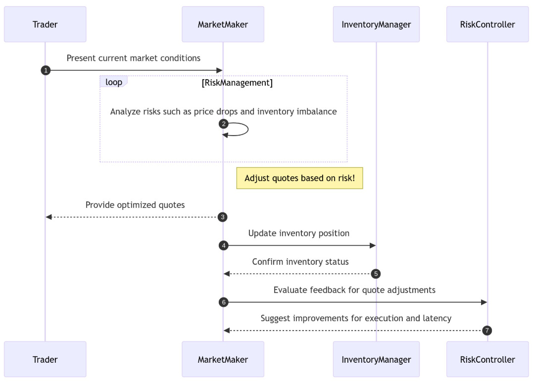
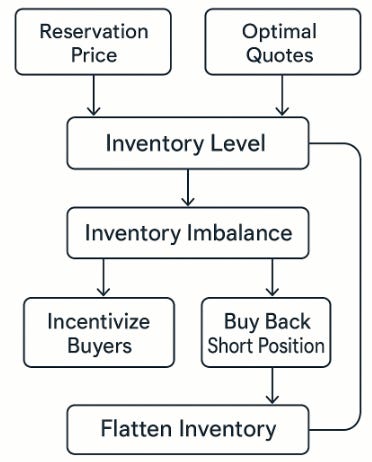
Inventory management dynamics
The model essentially turns inventory management into a feedback control system. Your current inventory level is the system's state variable, and the reservation price and optimal quotes are the control signals designed to steer that state towards zero.
Imagine inventory as a boat's ballast. Too much ballast on one side—long inventory— and the boat lists, becoming unstable. The market maker's strategy, guided by the lower reservation price and willingness to sell, is to effectively jettison some of that ballast by incentivizing buyers. Conversely, too little ballast or ballast skewed to the other side—short inventory—and the boat lists the other way. The strategy then shifts to buying back the short position.
The beauty is in the dynamic nature. The pressure to flatten inventory isn't constant; it intensifies as the end of the trading horizon approaches. As (T−t) shrinks, the inventory risk adjustment still depends on q, γ, and σ2, but the multiplier of that risk (T−t) decreases. However, simultaneously, the risk component of the spread also shrinks, potentially narrowing the spread based on this component. This creates a nuanced interplay. While the per-unit inventory pain might feel less intense as time runs out, the urgency to flatten before the horizon ends— t=T, where the model assumes inventory must be zeroed out or its value is simply q×S—means the quotes will still aggressively try to attract offsetting trades if inventory is significantly non-zero.
The model implicitly pushes for higher trading volume when inventory is imbalanced and time is running out, even if it means quoting slightly less profitable prices relative to the mid-point. This constant push and pull—between seeking profitable spreads and managing inventory risk—is the core dynamic orchestrated by the reservation price.
Avellaneda-Stoikov Implementation
Quants have developed sophisticated variations that address some of these issues, incorporating jump-diffusion processes for prices, more detailed order book dynamics, and transaction costs. Nevertheless, the basic Avellaneda–Stoikov framework provides the essential conceptual bedrock upon which these more complex models are built.
Let’s code it in its basic form: