

[WITH CODE] Data: Iceberg orders
Market makers exploit unseen order patterns, tipping the scales in high-frequency trading battles

Table of contents:
Introduction.
What are iceberg orders?
Finite state machine for native icebergs.
Detection of synthetic icebergs.
Kaplan–Meier estimation.
Who benefits from iceberg order detection?
Before you begin, remember that you have an index with the newsletter content organized by clicking on “Read the newsletter index” in this image.

Introduction
Welcome to the golden age of finance, where trading platforms promise to turn your pocket change into a private jet—or at least a slightly nicer bicycle—using algorithms that apparently outperform Wall Street geniuses and basic math. Between the risk-free strategies that evaporate faster than your patience during a software update… a darker color scheme, it’s clear innovation here means inventing new ways to monetize your FOMO.
I'm talking about a specific company: #00k!@? I was browsing their website for some really cool photos with balloons and came across an interesting section. It's about the iceberg orders section—the rest, I have to say, is okay, not bad for a discretionary retailer. This made me ask myself a few questions like for example: Does it really make sense to invest time and computational resources in detecting iceberg orders?
The answer is nuanced. On one hand, for certain players—like HFT firms and market makers—knowledge about hidden liquidity can be invaluable. On the other hand, the complexity and inherent uncertainty in detecting synthetic icebergs may limit the practical benefit of these methods in a fast-moving trading environment. Furthermore, the reliance on historical order book data means that real-time implementation may require substantial adaptation.
What are iceberg orders?
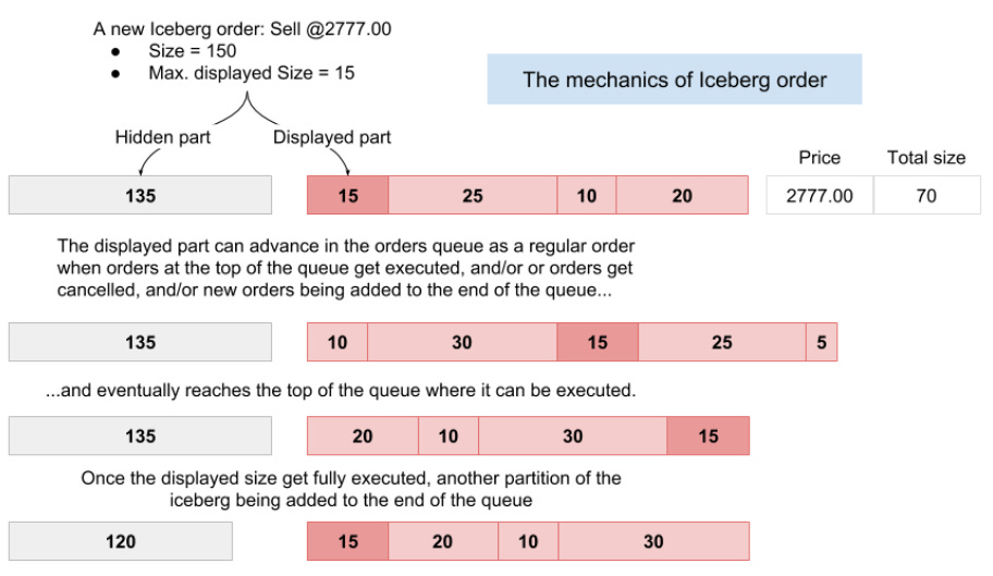
Basically, it is a type of limit order used to hide the true trading intention of a participant. Instead of revealing the full order size, only a peak amount is visible in the order book. When this peak is executed, another tranche—or refill—is automatically submitted until the total volume is traded. The hidden volume remains concealed from the market, allowing large traders to minimize market impact. The term iceberg is used because, like a natural iceberg, the majority of the volume—the mass below the surface—is hidden from view.
The basic principle of how, for instance, Buy Iceberg orders operate is this:
The mechanics of Iceberg order matching is quite similar except that only its displayed size can advance in the order queue.
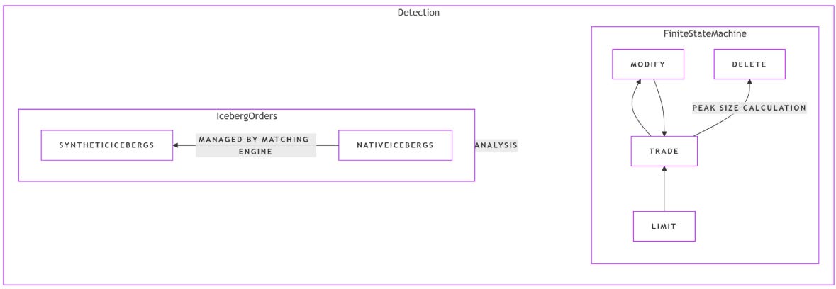
With this in mind, we can check the two types of iceberg orders. They come in two flavors:
Native icebergs: Managed by the exchange’s matching engine, they exhibit telltale characteristics such as a constant order ID and trade summary messages that sometimes indicate trade volumes larger than the current visible order size.
Synthetic icebergs: Managed by external systems—typically independent software vendors, or ISVs)—these orders are recreated by submitting multiple limit orders with the same price and volume characteristics. Their detection relies on time-based heuristics, as the exchange does not provide explicit markers.
You can see more about that in the work of Frey and Sandås:
To date, many methodologies have been attempted for its detection, each more eccentric than the last. Some firms have used analytical models, others claim to use ML—but in the end, we're talking about linear regression. It's all possible. Let's look at some of these applications and what the industry is using to model this chimera.
Finite state machine for native icebergs
For native iceberg orders, the detection algorithm tracks the order’s lifecycle. A new limit order enters the book, may be partially executed, and then gets updated or refilled with additional volume until it is either fully executed or cancelled. We can formally define the finite state machine as follows:
Let S={L,T,M,D} denote the set of states:
L: Limit—order appears in the book.
T: Trade—execution against the order.
M: Modify—refill or update indicating additional hidden volume.
D: Delete—order leaves the book.
Define a state transition function
where A is the set of order actions—Limit, Trade, Modify, Delete. The transitions are governed by the following rules:
δ(L,Trade)=T.
δ(T,Modify)=M.
δ(M,Trade)=T.
δ(T,Delete)=D.
δ(M,Delete)=D.
A typical sequence for an iceberg order is:
Let’s see an example of how to make the computations for Peak Size. Consider an order that follows this sequence:
A limit order with volume VL=6.
A trade occurs with volume VT=12.
The order is modified aka refilled with a new visible volume VM=7.
The peak size Vpeak is defined by the relation:
where k∈N0 is the number of complete tranches executed prior to the current modification.
For instance, if k=1—indicating that one complete tranche has been executed—then
This indicates that if the next refill is equal to 9, the order confirms the iceberg pattern.
This table illustrates a simplified sequence:
Beyond these basic computations, one may consider the cumulative traded volume after i trades and the corresponding sequence of modifications. Formally, if
where vj is the volume traded in the j-th trade, then the admissible peak sizes satisfy
Personally, a finite state machine seems pretty toyish to me. Sometimes I wonder to what extent firms will use this... but anyway, let's implement it.

Feel free to adjust or expand this to suit your own environment and order logic.
import enum
class OrderState(enum.Enum):
"""
Order states for a native iceberg:
- L: Limit (the order is live on the book with some visible size)
- T: Trade (the order experiences a trade / fill event)
- M: Modify (the order is modified or refilled)
- D: Delete (the order is removed or canceled)
"""
L = "Limit"
T = "Trade"
M = "Modify"
D = "Delete"
class IcebergOrder:
"""
A simple class modeling a native iceberg order using a state machine.
Attributes:
initial_visible (float): The initial visible portion of the iceberg.
total_volume (float): The total size of the iceberg (visible + hidden).
state (OrderState): The current state of the order.
traded_volume (float): How much volume has been traded so far.
completed_tranches (int): Number of times the visible portion has been fully filled.
Methods:
trade(volume): Simulate a trade (fill) of 'volume'.
modify(new_visible): Simulate a modification of the order's visible portion.
delete(): Cancel (delete) the order.
refill(): Automatically refill the visible portion if hidden volume remains.
compute_peak_size(): Recompute the new peak size based on the example formula.
step_through_sequence(): Demonstration of a typical L -> T -> M -> T -> ... -> D flow.
"""
def __init__(self, initial_visible: float, total_volume: float):
self.initial_visible = initial_visible
self.total_volume = total_volume
self.state = OrderState.L
# Tracking volumes:
self.visible_volume = initial_visible
self.hidden_volume = max(total_volume - initial_visible, 0.0)
self.traded_volume = 0.0
self.completed_tranches = 0
def trade(self, volume: float):
"""
Simulate a trade (fill) of 'volume' units.
Transitions state to T (Trade).
"""
if self.state == OrderState.D:
print("Order is deleted, cannot trade.")
return
self.state = OrderState.T
# Actual traded amount is limited by the visible volume
fill = min(self.visible_volume, volume)
self.visible_volume -= fill
self.traded_volume += fill
print(f"[TRADE] Filled {fill} units. "
f"Remaining visible = {self.visible_volume}, "
f"Traded so far = {self.traded_volume}")
# If visible is fully filled, we count a completed tranche
if self.visible_volume <= 0.0:
self.completed_tranches += 1
# Attempt to refill if hidden volume remains
self.refill()
def modify(self, new_visible: float):
"""
Simulate modifying the order's visible portion.
Transitions state to M (Modify).
"""
if self.state == OrderState.D:
print("Order is deleted, cannot modify.")
return
self.state = OrderState.M
# Adjust the visible portion (within what remains in the hidden volume)
# For demonstration, just set it to new_visible (bounded by hidden).
self.visible_volume = min(new_visible, self.hidden_volume + self.visible_volume)
self.hidden_volume = self.total_volume - self.traded_volume - self.visible_volume
print(f"[MODIFY] New visible portion set to {self.visible_volume}. "
f"Hidden volume is now {self.hidden_volume}.")
def delete(self):
"""
Delete (cancel) the order.
Transitions state to D (Delete).
"""
self.state = OrderState.D
print("[DELETE] Order is deleted.")
def refill(self):
"""
If the visible portion has been completely filled,
try to refill from the hidden portion (iceberg logic).
Typically triggers a Modify state, but we can automate here.
"""
if self.hidden_volume > 0.0:
# Move to modify state to refill
self.state = OrderState.M
# Compute the new peak size (example formula) or just use initial_visible
new_peak = self.compute_peak_size()
# The new visible portion is the smaller of new_peak or what's left hidden
refill_amount = min(new_peak, self.hidden_volume)
self.visible_volume = refill_amount
self.hidden_volume -= refill_amount
print(f"[REFILL] Refilled visible portion to {self.visible_volume}. "
f"Hidden volume is now {self.hidden_volume}.")
# After modifying, we can switch back to 'L' to indicate it's a valid limit again
self.state = OrderState.L
else:
# No more hidden volume left -> entire order is filled
print("[REFILL] No hidden volume left. The order is fully executed.")
self.delete()
def compute_peak_size(self) -> float:
"""
Compute the new peak size using the example formula:
V_peak = (traded_volume + initial_visible) / (completed_tranches + 1)
This is just one interpretation from your example.
"""
if self.completed_tranches == 0:
# If no tranches have completed, just return the initial visible
return self.initial_visible
# Example formula from your snippet:
# V_peak = (V_T + V_L) / (k + 1)
# Where k is the number of completed tranches so far
return (self.traded_volume + self.initial_visible) / (self.completed_tranches + 1)
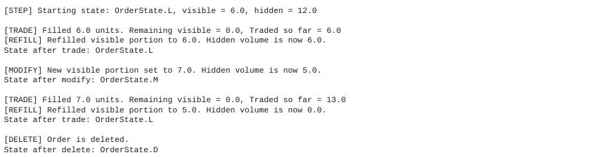
def step_through_sequence(self):
"""
Demonstration of a typical sequence:
L -> T -> M -> T -> ... -> D
You can tailor these steps to your actual use case.
"""
print(f"\n[STEP] Starting state: {self.state}, "
f"visible = {self.visible_volume}, hidden = {self.hidden_volume}\n")
# 1) Trade event
self.trade(6.0) # Suppose a partial fill of 6
print(f"State after trade: {self.state}\n")
# 2) Modify event (change the visible portion)
self.modify(7.0)
print(f"State after modify: {self.state}\n")
# 3) Another trade event
self.trade(12.0) # Another fill
print(f"State after trade: {self.state}\n")
# 4) Finally, delete the order
self.delete()
print(f"State after delete: {self.state}\n")
def main():
# Example usage:
# Create an iceberg order with an initial visible volume of 6 and total volume of 18
iceberg = IcebergOrder(initial_visible=6.0, total_volume=18.0)
# Show a demonstration sequence
iceberg.step_through_sequence()
if __name__ == "__main__":
main()Your output must be:
You can tailor:
The peak-size logic to match your exact refill strategy.
The sequence of trades and modifications to reflect your real-world use cases.
Any additional constraints—e.g., partial refills, partial modifies, multi-step trades.
Detection of synthetic icebergs
Unlike native icebergs, synthetic icebergs lack a persistent order ID. Instead, they are detected using a timing heuristic. Suppose that when a limit order is cancelled or fully executed, a new limit order with identical price P and volume V is submitted within a short time interval dt. Formally, let
and if Δt≤dt—e.g., dt=0.3 seconds—then the new order is considered part of the same iceberg chain.
When multiple candidate orders are present, the algorithm selects the one with the minimum Δt. If there exist hhh candidate chains, a weighting scheme is applied:
for the i-th iceberg tree. The total volume Vtotal of the iceberg can be aggregated in several ways:
Average total volume of all chains:
\(\hat{V}_{\text{all}} = \frac{1}{h_i} \sum_{\ell=1}^{h_i} V_{i,\ell},\)Average total volume of chains of unique length:
\(\hat{V}_{\text{unique}} = \frac{1}{|H|} \sum_{\ell \in H} V_{i,\ell},\)where H denotes the set of chains with unique lengths.
Total volume of the longest chain:
\(\hat{V}_{\text{longest}} = \max_{\ell=1,\dots,h_i} V_{i,\ell}.\)
Once again feel free to adjust the details:
import math
from typing import List, Dict, Any
class SyntheticIcebergDetector:
"""
Detects synthetic iceberg orders based on:
- Same (price, volume) criteria
- Time proximity (dt <= dt_threshold)
- If multiple chains are possible, choose the chain with the highest weight
w_i = 1 / h_i (i.e., the chain with the fewest orders so far).
After detection, computes aggregate stats:
- Average total volume of all chains
- Average total volume of chains of unique length
- Total volume of the longest chain
"""
def __init__(self, dt_threshold: float = 0.3):
"""
Args:
dt_threshold: Maximum time gap (in seconds) to consider
consecutive orders as part of the same chain.
"""
self.dt_threshold = dt_threshold
def detect(self, orders: List[Dict[str, Any]]) -> List[List[Dict[str, Any]]]:
"""
Main detection function. Groups orders into chains.
Each order is expected to have at least:
{
'time': float or numeric (timestamp),
'price': float,
'volume':float,
# optionally 'side': 'BUY'/'SELL' if needed
}
Returns:
A list of chains, where each chain is a list of order dicts.
"""
# 1) Sort orders by time
orders_sorted = sorted(orders, key=lambda x: x['time'])
# 2) We'll store chains as a list of lists
# each chain = [order1, order2, ...]
chains = []
for order in orders_sorted:
# Check if this order can belong to one (or more) existing chain(s)
candidate_chains = []
for chain_idx, chain in enumerate(chains):
last_order = chain[-1]
# Check if it matches the (price, volume) (and optionally side)
same_price_vol = (
math.isclose(last_order['price'], order['price']) and
math.isclose(last_order['volume'], order['volume'])
)
# If you want to match side as well, uncomment below:
# same_price_vol = same_price_vol and (last_order['side'] == order['side'])
# Check time difference
dt = order['time'] - last_order['time']
if same_price_vol and (0 <= dt <= self.dt_threshold):
# This chain is a valid candidate
candidate_chains.append(chain_idx)
if not candidate_chains:
# Start a new chain
chains.append([order])
else:
# If multiple candidates, pick the one with the highest weight w_i = 1/h_i
# => the chain with the smallest current length h_i
best_chain_idx = min(candidate_chains, key=lambda idx: len(chains[idx]))
chains[best_chain_idx].append(order)
return chains
def compute_aggregates(self, chains: List[List[Dict[str, Any]]]) -> Dict[str, float]:
"""
Compute:
1) 'average_all': average total volume across all chains
2) 'average_unique': average total volume of chains whose length is unique
3) 'longest_chain_volume': total volume of the longest chain (by volume)
Returns:
Dictionary with keys: 'average_all', 'average_unique', 'longest_chain_volume'
"""
# 1) Compute total volume of each chain
chain_volumes = []
chain_lengths = []
for chain in chains:
# total volume = sum of volumes in that chain
total_vol = sum(o['volume'] for o in chain)
chain_volumes.append(total_vol)
chain_lengths.append(len(chain))
n_chains = len(chains)
if n_chains == 0:
return {
'average_all': 0.0,
'average_unique': 0.0,
'longest_chain_volume': 0.0
}
# 1) Average total volume of all chains
average_all = sum(chain_volumes) / n_chains
# 2) Average total volume of chains of *unique* length
# We only include chains whose length h_i is "unique" among all chain lengths.
length_counts = {}
for L in chain_lengths:
length_counts[L] = length_counts.get(L, 0) + 1
# Identify chain indices that have a unique length
unique_chain_indices = [
i for i, L in enumerate(chain_lengths)
if length_counts[L] == 1
]
if len(unique_chain_indices) > 0:
average_unique = (
sum(chain_volumes[i] for i in unique_chain_indices)
/ len(unique_chain_indices)
)
else:
average_unique = 0.0
# 3) Total volume of the "longest" chain
# We interpret "longest" as the chain with the greatest total volume
longest_chain_volume = max(chain_volumes)
return {
'average_all': average_all,
'average_unique': average_unique,
'longest_chain_volume': longest_chain_volume
}
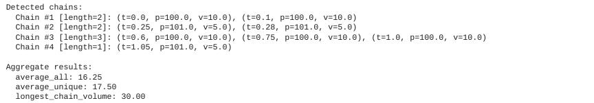
def demo():
"""
A small demo showing how to use the SyntheticIcebergDetector.
"""
# Example data: list of orders
# Each order has (time, price, volume).
# We'll keep times simple (floats) for the example.
orders = [
{'time': 0.00, 'price': 100.0, 'volume': 10.0},
{'time': 0.10, 'price': 100.0, 'volume': 10.0},
{'time': 0.25, 'price': 101.0, 'volume': 5.0},
{'time': 0.28, 'price': 101.0, 'volume': 5.0},
{'time': 0.60, 'price': 100.0, 'volume': 10.0},
{'time': 0.75, 'price': 100.0, 'volume': 10.0},
{'time': 1.00, 'price': 100.0, 'volume': 10.0},
{'time': 1.05, 'price': 101.0, 'volume': 5.0},
]
detector = SyntheticIcebergDetector(dt_threshold=0.3)
chains = detector.detect(orders)
print("Detected chains:")
for i, chain in enumerate(chains, start=1):
chain_desc = ", ".join(
f"(t={o['time']}, p={o['price']}, v={o['volume']})"
for o in chain
)
print(f" Chain #{i} [length={len(chain)}]: {chain_desc}")
results = detector.compute_aggregates(chains)
print("\nAggregate results:")
for k, v in results.items():
print(f" {k}: {v:.2f}")
if __name__ == "__main__":
demo()The output looks like this:
For this method there are things you need to take into account:
You may also want to consider the side of the order if that’s relevant—i.e., only chain up buy orders with buy orders, etc.
If your environment or data feed has different time formats—e.g. datetime strings—convert them to numeric timestamps before sorting.
The weighting scheme wi=1/hi.

Kaplan–Meier estimation
To predict the full size of an iceberg order, the Kaplan–Meier estimator is used to account for censored data—e.g., cancelled orders. For a given peak size p, let Vp be the random variable representing the total volume of an iceberg with peak p. The survival function is defined as:
where Fp(v)=Pr(Vp≤v) is the cumulative distribution function.
Given a sorted set of unique volume levels {u1,u2,…,uK}, let:
dp be the number of complete events—iceberg completions—at volume uj,
nj be the number of orders at risk at volume uj.
The Kaplan–Meier estimator is then:
An extension involves the hazard function λp(v), defined as:
In discrete settings, the hazard rate at uj can be approximated by:
For synthetic icebergs, the estimator is modified using weighted counts:
Thus, the weighted Kaplan–Meier estimator becomes:
This formulation allows us to compute not only the survival probabilities but also to derive the probability mass function (pmf) for Vp by:
ensuring that the total probability sums to 1 after proper normalization.
Let’s see how to implement this other one. In practical terms, this code can be used to estimate a survival function for the random variable—the peak size—and then derive the corresponding probability mass function.