[WITH CODE] Model: Online clustering

Sequential online K-Means algorithm

Jun 30, 2025

∙ Paid

Table of contents:

Introduction.
Risk and limitaitons of online models.
Batch K-Means
Introducing the online paradigm.
Initialization and path dependency.
The curse of dimensionality and search optimization.
Evaluating performance on a moving target.
From clusters to signals.

Before you begin, remember that you have an index with the newsletter content organized by clicking on “Read full story” in this image.

Introduction

Alright team, let’s dive deeper into something we've all painfully experienced: You spend days meticulously crafting a K-Means clustering model—furthermore, you have decided to use it incorrectly to classify market regimes instead of applying it to other processes. The backtest results look flawless—you're confident and ready.

But then, the model goes live, and within weeks, your PnL starts bleeding heavily. So, what happened? Simply put, markets aren't static—or simply, that application to identify market regimes is nonsense. But ok, let's proceed with the same example: what was confidently classified as high volatility last quarter might now merely be background noise. That perfect momentum regime you painstakingly identified suddenly fractures into several distinct new states, and your static model has no clue how to adjust.

We've all seen it: those carefully crafted clusters that once captured clear market states now blur and shift unpredictably. Economic reports, central bank decisions, sudden geopolitical tensions, or even subtle changes in investor sentiment can swiftly redefine the landscape. Relying on static clusters is like trying to catch lightning in a bottle—it might look great initially, but inevitably, you end up chasing shadows.

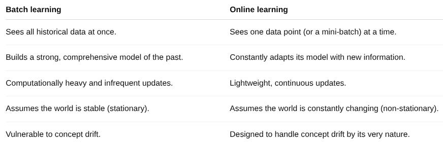
Here's the crux of the issue: traditional batch clustering—the type that demands your entire historical dataset upfront—assumes a world frozen in time. Imagine navigating today's Manhattan with a detailed street map from the 1990s. The broad outlines and main avenues might still be correct, sure, but navigating the intricate, constantly evolving details—like new skyscrapers, blocked roads, and changing traffic flows—is nearly impossible. You'll end up lost, frustrated, and far from your destination.

In financial markets, this analogy couldn't be more accurate. New market participants, technological advancements, regulatory shifts, and evolving trading strategies constantly reshape the market terrain. Static models, anchored to historical datasets, rapidly lose their relevance, becoming not just inaccurate but potentially hazardous. They can mislead your strategies, resulting in positions that are poorly aligned with current market conditions, thus amplifying risks and eroding profits.

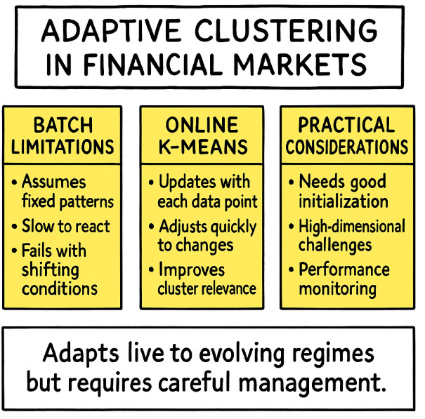
That’s exactly why Sequential Online K-Means isn't merely an incremental improvement—it's a fundamentally different, smarter way of thinking. Unlike batch methods, it doesn’t rely on outdated snapshots. Instead, Sequential Online K-Means is dynamic, learning and adapting continuously with each incoming data point. Think of it as a real-time heartbeat monitor, updating its understanding of market regimes tick by tick, trade by trade, and responding promptly to subtle shifts and significant shocks alike.

This approach doesn't just enhance performance; it aligns with the very nature of financial markets. As new trades occur, Sequential Online K-Means recalibrates its clusters, ensuring they accurately reflect the current market regime. It adapts quickly during periods of volatility, swiftly integrating new data to refine its regime classifications, thereby providing more reliable, timely, and actionable insights.

Let's be clear: we're not just refining an existing method; we’re addressing a fundamental misalignment between how batch algorithms view the market and how markets truly operate. This constant flux demands models that can flex and adjust with similar speed and sensitivity.

Risk and limitaitons of online models

Online models, including sequential k-means, offer the ability to learn from data streams in real time, but they come with a distinct set of risks and limitations that are crucial to understand.

Since online models learn sequentially, a model trained on past data may become inaccurate as the underlying data distribution shifts. This can happen suddenly (e.g., due to a market crash) or gradually (e.g., changes in customer behavior).
Errors in online learning can compound. If the model makes a mistake, that incorrect learning can influence future updates, potentially leading the model to drift further from an accurate state. Unlike batch models that can correct themselves with a global view of the data during retraining, online models have a more localized and sequential perspective.
While online models don't need to hold all historical data in memory, they must be fast enough to process incoming data points without falling behind. This can be a challenge in high-throughput environments, and the computational resources required can be a limiting factor.
Assessing the performance of an online model is more complex than for a batch model. There is no fixed test set. Evaluation must be done continuously on new, incoming data, making it difficult to get a stable measure of the model's accuracy. This requires robust monitoring and the ability to distinguish between model degradation and normal fluctuations in the data.

Batch K-Means

Let's get down to brass tacks. The problem with batch clustering, specifically K-Means, isn't a subtle philosophical point; it's a mathematical one. The algorithm's objective is to solve an optimization problem. Given a dataset X={x₁,x₂,...,x_N}, we want to find a set of k centroids C={c₁,c₂,...,c_k} that minimizes the inertia, or the within-cluster sum-of-squares.

Mathematically, we are trying to find:

\(\arg\min_{C} \sum_{j=1}^{k} \sum_{x_i \in S_j} \big\lVert x_i - c_j \big\rVert^2\)

Where S_j is the set of all data points xi assigned to cluster j, and c_j is the centroid of that cluster—typically the mean of all points in S_j.

The standard algorithm to solve this—Lloyd's algorithm—is an iterative process:

Initialization: Pick k initial centroids.
Assignment step: Assign each data point x_i to its nearest centroid.
Update step: Recalculate each centroid c_j as the mean of all points assigned to it.
Repeat: Repeat steps 2 and 3 until the assignments no longer change.

Notice the implicit assumption here. The entire dataset X must exist and be held in memory for this to work. The update step computes the mean across all points assigned to a cluster. This is the definition of a batch process. It presumes the world is a closed system, a finished book. In finance, we're lucky if we have the current page, and we know for a fact the next one is being written as we speak.

This leads to two critical failures in a financial context:

Covariate shift: It is the milder of the two. The distribution of our input features—covariates—changes, but the underlying relationship between inputs and outputs—the concept—remains the same. For example, the average daily trading volume might increase across the market, but the patterns that define a momentum regime might still hold. A batch model will struggle because its sense of scale is now off.
Concept drift: It is the true killer. The fundamental relationship we are trying to model changes. The very definition of a volatile market regime might change. What was considered high volatility in 2017 might be considered moderate in 2025. A model trained on the old concept is now fundamentally broken.

You can check more about batch clustering here:

Trading the Breaking

[WITH CODE] Model: Clustering

a year ago · 17 likes · 𝚀𝚞𝚊𝚗𝚝 𝙱𝚎𝚌𝚔𝚖𝚊𝚗

The batch model is blind. It has no mechanism to create a new cluster or even significantly adjust its existing ones. It simply shoehorns new reality into its old, rigid framework. This is the tyranny of the batch: forcing a dynamic process into a static representation.

To visualize this failure, we can use a simple plot. Imagine the red and blue clusters are our historical data. The batch model finds their centers—the black X's. Then, a new green cluster appears. The batch model has no choice but to misclassify all the green points as belonging to the blue cluster, because its structure is frozen.

Introducing the online paradigm

If batch processing is a photograph, online learning is a live video feed. It processes the world frame by frame, or in our case, data point by data point.

The algorithm we're interested in, often called Sequential K-Means or Online K-Means, is a beautiful adaptation of the batch concept. It essentially performs a mini-update every time it sees a new piece of data.

Initialization and path dependency

We've established that an online model is like a living thing, its state evolving over time. But this raises a crucial, almost philosophical question: what about its birth? The initial state of the centroids is not a trivial detail. Because the model updates sequentially, its entire life story—its path through the feature space—is heavily influenced by where it started.

This is path dependency, the ghost in the online machine. A poor initialization can send the centroids down a garden path from which they may never find their way to the globally optimal positions.

Imagine two market regimes that are quite distinct but start close together in the feature space. If we randomly initialize two centroids and one happens to land right between these two budding regimes, it might get stuck, incorrectly representing both and never allowing two distinct clusters to form. Another centroid, initialized far away in an empty region of the space, might become a "dead" cluster, never attracting any points.

This is the cold start problem. We need a way to initialize our centroids intelligently, to give our model the best possible start in life. The naive approach is simple random sampling: pick k data points from our initial chunk of data and call them centroids. It's fast, but it's also dumb luck.

A much smarter approach is K-Means++. The intuition behind K-Means++ is to place initial centroids far away from each other. It's a probabilistic algorithm that aims for good spatial separation.

The process is as follows:

Choose the first centroid c₁ uniformly at random from the initial data points X_init.
For each subsequent centroid i=2,...,k:
1. For each data point x∈X_init, calculate D(x), the distance from x to the nearest already-chosen centroid.
2. Choose the next centroid ci from the remaining data points with a probability proportional to D(x)².
  \(P(x) \;=\; \frac{D(x)^2}{\displaystyle\sum_{x' \in X_{\mathrm{init}}} D(x')^2} \)

Why D(x)²? Squaring the distance means that points far away from existing centroids have a much, much higher chance of being chosen as the next centroid. This actively encourages the algorithm to explore new, distant regions of the feature space for its initial placement. It's a greedy but incredibly effective heuristic.

Let's examine how our OnlineKMeans class implements this. It's right there in the _initialize_centroids method.

def _initialize_centroids(self, X: np.ndarray) -> None:
    if self.init == "kmeans++":
        # 1. Choose the first centroid randomly
        centroids = [X[self.rng.integers(len(X))]]
        for _ in range(1, self.n_clusters):
            # 2a. Calculate D(x)^2 for all points
            dist_sq = np.min(
                [np.sum((X - c) ** 2, axis=1) for c in centroids], axis=0
            )
            # 2b. Choose next centroid with probability proportional to D(x)^2
            probs = dist_sq / dist_sq.sum()
            idx = self.rng.choice(len(X), p=probs)
            centroids.append(X[idx])
        self.centroids = np.vstack(centroids)
    else: # The 'random' option
        indices = self.rng.choice(len(X), size=self.n_clusters, replace=False)
        self.centroids = X[indices].copy()

    self.counts = np.zeros(self.n_clusters, dtype=int)

The code is a direct translation of the algorithm. It iteratively builds up the list of centroids, and for each new one, it calculates the squared distances (dist_sq), normalizes them to form a probability distribution (probs), and then makes a weighted random choice (rng.choice).

The impact of this is enormous. By starting with well-separated centroids, the model is less likely to get stuck in local minima. Each initial centroid is more likely to be near the "true" center of a distinct data cloud. This gives the online learning process a massive head start, ensuring the path it takes is a productive one.

K-Means++ plot will show a more stable and accurate evolution. It's the difference between starting a marathon in the right stadium versus in a neighboring city.

The curse of dimensionality and search optimization

In our online algorithm, we have a loop that runs for every single data point. And inside that loop, the very first step is _closest_centroid(x). This is the workhorse of the entire process. For every tick of market data, we must compare it to all k of our current centroids to find the winner.

If we do this naively, it's a brute-force search. We calculate the distance from our new point x to c₁, then to c₂, and so on, up to ck. If our data is in a d-dimensional feature space, the cost of one distance calculation is O(d). Since we do this k times, the total cost to assign one point is O(k⋅d).

For a small number of clusters and low-dimensional data, this is perfectly fine. If we're clustering based on 2 features into 5 regimes, the cost is negligible. But in quantitative trading, we often work with high-dimensional feature spaces. We might use dozens of features: various moving averages, volatility measures, order book imbalances, sentiment scores, etc.

Let's say we have d=50 features and we're looking for k=30 market regimes. The cost starts to add up. More importantly, it scales linearly with the number of clusters. If we want to test a model with 100 clusters, our assignment step just got over 3 times slower. In a high-frequency context where we need to process thousands of updates per second, this linear scaling can become a critical bottleneck.

This is where clever data structures come to the rescue. We don't have to check every single centroid. If we can structure our centroids in a way that allows for faster searching, we can gain a significant speed advantage. The most common structure for this is a KD-Tree—K-Dimensional Tree.

A KD-Tree is a binary tree that recursively partitions the feature space. At each level of the tree, it picks one dimension—often cycling through them—and finds the median point along that dimension. It then splits the data into two halves based on that median, which become the left and right children in the tree. The result is a hierarchical partitioning of the space into nested rectangular hyperregions.

When we want to find the nearest neighbor—our closest centroid—for a new point x, we traverse the tree down to the leaf node where x would belong. This gives us an initial guess for the closest centroid. The magic of the KD-Tree is that we can then backtrack up the tree, and for each parent node, we only need to explore the other branch if it's possible it could contain a point closer than our current best. Often, we can prune entire branches of the search space, ruling out many centroids without ever calculating the distance to them.

The average time complexity for a nearest-neighbor search in a KD-Tree is O(d⋅log k). Compare that to the brute-force O(k⋅d). The logarithm is a powerful thing. If we have k=100 clusters, log₂(100) is about 6.64. The KD-Tree search could be more than an order of magnitude faster than the brute-force approach.

However, there's no free lunch.

Building the KD-Tree in the first place has a cost, typically O(k⋅log k). Since our centroids are moving, we can't just build it once. We have to rebuild it periodically.
KD-Trees work brilliantly in low dimensions. But as the number of dimensions d gets very large, their performance degrades and can become even worse than brute-force. The concept of distance becomes less meaningful, and most points become roughly equidistant.
If the number of clusters k is very small, the overhead of building and traversing the tree might be greater than the cost of a simple brute-force search.

Our OnlineKMeans class handles this trade-off with two parameters: index_rebuild_freq and index_threshold.

class OnlineKMeans:
    def __init__(self, ..., index_rebuild_freq: int = 50, index_threshold: int = 20):
        # ...
        self.index_rebuild_freq = index_rebuild_freq
        self.index_threshold = index_threshold
        self._nn_index: Optional[NearestNeighbors] = None

    def _build_nn_index(self) -> None:
        # Don't build an index if k is too small.
        if self.n_clusters < self.index_threshold:
            self._nn_index = None # This signals to use brute-force
            return

        # Use scikit-learn's NearestNeighbors, which can build a KD-Tree
        self._nn_index = NearestNeighbors(n_neighbors=1, algorithm="auto")
        self._nn_index.fit(self.centroids)

    def _closest_centroid(self, x: np.ndarray) -> int:
        if self._nn_index is None: # Use brute-force
            dists = np.linalg.norm(self.centroids - x, axis=1)
            return int(np.argmin(dists))
        else: # Use the pre-built index
            idx = self._nn_index.kneighbors(x.reshape(1, -1), return_distance=False)
            return int(idx[0, 0])

    def fit(self, X: np.ndarray) -> None:
        # ...
        for i, x in enumerate(X):
            # ... update logic ...
            # Rebuild the index occasionally
            if (i + 1) % self.index_rebuild_freq == 0:
                self._build_nn_index()

This is a pragmatic and robust implementation. The index_threshold says don't bother with fancy indexing unless we have at least 20 clusters. The index_rebuild_freq says the centroids are moving, so to keep our search structure accurate, throw away the old one and build a new one every 50 data points. This prevents the index from becoming stale while not incurring the cost of rebuilding it on every single update.

Send me a copy

Evaluating performance on a moving target

We've built an adaptive clustering machine. It hums along, consuming market data and shifting its centroids. But a crucial question remains: is it any good? In batch learning, evaluation is straightforward. We have a static dataset and static labels. We can compute metrics like accuracy, precision, recall, or, in the case of clustering, inertia and the silhouette score. With an online model, the ground truth is a moving target. The very concept drift we're trying to capture means that there's no fixed set of correct clusters.

This is the Oracle's Dilemma. We can't ask an all-knowing oracle for the true labels at each time step. We need to evaluate the model using only the data it has seen and the structure it has created. This means we must rely on internal validation metrics. These metrics assess the quality of the clustering based solely on the geometry of the clusters themselves.

The two most common metrics are Inertia and the Silhouette Score.

Inertia aka Within-Cluster Sum of Squares: We've already met this one. It's the objective function that K-Means tries to minimize.

\(I \;=\; \sum_{j=1}^{k} \sum_{x_i \in S_j} \bigl\lVert x_i - c_j \bigr\rVert^2. \)

In an online context, we can track the inertia over a rolling window of recent data. A lower inertia is generally better, indicating that the points are, on average, closer to their assigned centroids. A sudden spike in inertia is a red flag. It could mean that our centroids are no longer representative of the incoming data—a clear sign of concept drift.

Silhouette score: This is a more sophisticated and often more insightful metric. It measures how well-separated and dense the clusters are. For each data point x_i, the silhouette score s(i) is calculated:

\(s(i) \;=\; \frac{b(i) - a(i)}{\max\bigl(a(i),\,b(i)\bigr)}.\)

Let's break down the terms:

a(i): The mean intra-cluster distance. This is the average distance from x_i to all other points within the same cluster. It's a measure of how tightly packed the cluster is. A small a(i) is good.
b(i): The mean nearest-cluster distance. This is the average distance from xi to all the points in the nearest neighboring cluster—the cluster that x_i is not a part of, but is closest to. A large b(i) is good.

The score s(i) ranges from -1 to 1:

Near +1: Indicates that the point is far from the neighboring cluster and very close to the other points in its own cluster. This is the ideal case. (a(i)≪b(i))
Near 0: Indicates that the point is on or very close to the decision boundary between two neighboring clusters. (a(i)≈b(i))
Near -1: Indicates that the point is probably misclassified and is closer to the points in a neighboring cluster than to its own. (a(i)>b(i))

The overall Silhouette Score for the model is the average of s(i) over all data points. A high score—e.g., > 0.5—suggests good, well-defined clusters. Tracking this score over time is key. A gradual decay in the Silhouette score can signal that the market regimes are becoming muddied or are starting to overlap. A sharp drop is a five-alarm fire; it strongly suggests a rapid regime change that has destroyed the existing cluster structure.

Let’s see how to implement this:

def silhouette_score(X: np.ndarray, labels: np.ndarray) -> float:
    # ...
    # Precompute the full N x N distance matrix. This is expensive!
    D = cdist(X, X)
    a = np.zeros(n_samples) # To store intra-cluster distances
    b = np.full(n_samples, np.inf) # To store nearest-cluster distances

    for lbl in unique:
        mask = labels == lbl
        # Calculate 'a' for all points in this cluster
        a[mask] = np.sum(D[np.ix_(mask, mask)], axis=1) / (cluster_size - 1)

        # Find the nearest other cluster to calculate 'b'
        for other in unique:
            if other == lbl: continue
            other_mask = labels == other
            # Mean distance from points in 'lbl' cluster to all points in 'other' cluster
            m = np.sum(D[np.ix_(mask, other_mask)], axis=1) / other_mask.sum()
            # We only care about the *nearest* other cluster, so we take the minimum
            b[mask] = np.minimum(b[mask], m)

    sil_values = (b - a) / np.maximum(a, b)
    return float(np.mean(sil_values))

Computing this on every single tick would be too slow due to the O(N²) distance matrix. In practice, we would compute it periodically (e.g., every few minutes) on a sliding window of the most recent N samples.