Portfolio: Portfolio of uncorrelated systems

Uncover the hidden dangers of correlated trading bots—before your portfolio pays the price

---

Table of contents:

1. Introduction.

2. Bots doing their homework.

3. The portfolio zoo—aka mix of bot strategies.

4. What are the dangers of having correlated bots?

5. Guide to building a portfolio of uncorrelated systems.

6. Balancing wins and losses.

---

Introduction

Trading bots are like the star players in a high-stakes orchestra—each with its own instrument, playing a unique tune. But when they’re all jamming together in the same portfolio, their harmony (or lack thereof) can either create a masterpiece or a cacophony. Today, we’re diving into the world of trading bots and how their interactions can make your portfolio sing or screech. The key idea? If bots move in sync, your portfolio can skyrocket or nosedive. But if they dance to their own beats, you’ll enjoy smoother, more predictable returns.

Let’s kick things off by decoding what a bot’s “PnL” really means and how to tell if two bots are best buddies or bitter rivals.

Bots doing their homework

In the trading world, PnL—Profit and Loss—is like a bot’s report card. It tells you how well the bot is performing. When we say two bots have correlated PnL, it means they tend to score high or low at the same time. This is measured using the correlation coefficient, denoted by ρ.

The correlation coefficient between two bots’ PnLs, PnL_A and PnL_B​, is calculated as follows:

\(\rho_{\mathrm{PnL}} = \frac{\mathrm{Cov}\bigl(\mathrm{PnL}_A, \mathrm{PnL}_B\bigr)}{\sigma_A \,\sigma_B} \)

Where:

• Covariance (Cov) measures how two variables move together.

• σ_A and σ_B are the standard deviations of the PnLs of Bot A and Bot B.

If ρ_PnL = 1, the bots are perfectly correlated—they move exactly in sync. If ρ_PnL = −1, they are perfectly anti-correlated—when one wins, the other hedge losses. And if ρ_PnL = 0, their moves are independent. Think of it like two classmates: sometimes they work together on a project—high correlation—and sometimes they work separately—zero correlation.

Our goal is for them to work independently, together but not mixed. The higher the correlation, the greater the risk. And a negative correlation can either be a real disaster or a well-coordinated portfolio of systems.

A simple example. Consider two bots:

• Bot A trades technology stocks.

• Bot B also trades technology stocks.

If both bots take a hit on the same day because of a tech crash, they’re highly correlated. But if one bot loses while the other gains—maybe by trading different sectors—they’re uncorrelated or even negatively correlated.

Now that we have defined PnL correlation, let’s look at how mixing different types of bots creates a diverse portfolio—much like mixing different flavors in a juice!

The portfolio zoo—aka mix of bot strategies

Different bots follow different strategies. Here are three common types:

• Arbitrage bot: The sneaky ninja of trading, exploiting tiny price differences between markets.

• Trend-following bot: The surfer, riding the waves of rising or falling markets.

• Mean-reversion bot: The bargain hunter, buying low and selling high when prices return to average.

When these bots have uncorrelated PnLs, combining them creates a robust portfolio. It’s like a zoo where lions, penguins, and sloths all contribute in their own unique ways. The result? Their risks don’t pile up destructively. And example here:

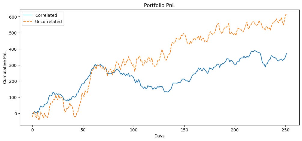
The cumulative PnLs are plotted to show how the portfolios perform over time. The uncorrelated portfolio is expected to be smoother, while the correlated one might exhibit more volatility.

After seeing how a mix of bots affects your portfolio’s performance, the next natural question is: What happens when all the bots decide to behave in the same way?

What are the dangers of having correlated bots?

When multiple bots chase the same market signals, their PnLs become highly correlated. This scenario is dangerous because it means that when one bot makes a mistake, all of them do. Think of it as a sports team where every player runs in the same direction—if that direction turns out to be wrong, the whole team suffers.

The variance of a portfolio consisting of N bots can be expressed as:

\(\sigma_p^2 = \sum_{i=1}^{N} w_i^2 \sigma_i^2 + 2 \sum_{i<j} w_i w_j \rho_{ij} \sigma_i \sigma_j \)

Here, w_i​ is the weight—or allocation—to bot i, σ_i​ is its standard deviation, and ρ_ij​ is the correlation between bots i and j.

• If ρ_ij ≈ 1 for all pairs:
  The second term adds up dramatically, making the portfolio extremely volatile. This is like building a tower out of jelly—it collapses easily!

Remember 2018? Several hedge funds using similar momentum strategies experienced massive losses because their bots acted in unison. When one bot dropped, others followed, and the losses compounded.

Knowing the dangers of highly correlated bots, let’s move to a practical guide on how to build an uncorrelated bot army. This is where the diversity of system typologies becomes your best friend—and by systems I don't mean vectors, but this is something we will cover in future articles.

Guide to building a portfolio of uncorrelated systems

Creating a portfolio of trading bots that do not mimic each other is the secret to reducing risk and ensuring smoother performance.

Step 1 - Different asset categories, different system categories:

In a robust portfolio:

• Bot A might trade technology stocks based on momentum.

• Bot B might focus on commodities based on trend following.

• Bot C might venture into cryptocurrency based on mean-reversion.

• Bot D might even trade exotic assets based on arbitrage.

Each bot follows its own strategy, ensuring that their PnLs are largely uncorrelated. In mathematical terms, this diversification minimizes the covariance terms in the portfolio variance equation.

Step 2 - Test historical correlations:

Before deploying a bot, you can measure how its PnL correlates with those of other bots. A common tool is the correlation matrix. The following code snippet shows how to calculate and visualize the correlation matrix:

import numpy as np
import pandas as pd
import matplotlib.pyplot as plt

# Set seed for reproducibility
np.random.seed(123)
days = 252  # Number of trading days in a year

# Generate PnLs for three different bots using a random walk
pnl_bot1 = np.cumsum(np.random.normal(1, 5, days))  # Arbitrage bot with drift
pnl_bot2 = np.cumsum(np.random.normal(1, 7, days) + 2 * np.sin(np.arange(days) / 20))  # Trend-following bot with noise
pnl_bot3 = np.cumsum(np.random.normal(1, 4, days) * (-1) ** np.random.randint(0, 2, days))  # Mean-reversion bot

# Generate a fourth bot that is correlated with Bot1 (80% mimicry with added noise)
pnl_bot4 = 0.8 * pnl_bot1 + np.cumsum(np.random.normal(0, 3, days))

# Combine the PnLs of the bots into a DataFrame
pnl_df = pd.DataFrame({
    'Bot1': pnl_bot1,
    'Bot2': pnl_bot2,
    'Bot3': pnl_bot3,
    'Bot4': pnl_bot4  # Note: Bot4 is correlated with Bot1
})

# Calculate the correlation matrix
corr_matrix = pnl_df.corr()

# Plot the correlation matrix using a heatmap
plt.figure(figsize=(8, 6))
plt.imshow(corr_matrix, cmap='coolwarm', vmin=-1, vmax=1)
plt.colorbar(label='Correlation coefficient')
plt.xticks(ticks=range(4), labels=pnl_df.columns)
plt.yticks(ticks=range(4), labels=pnl_df.columns)
plt.title("Bot PnL correlation matrix")
plt.show()

A heatmap displays the correlations, where red indicates high positive correlation and blue indicates low or negative correlation.

Step 3 - Deploy a correlation cop bot:

In practice, a portfolio manager might use a meta-bot or set rules that automatically adjust the capital allocation if two bots begin to show high correlation. The idea is to reduce the weight of bots that start copying each other.

For educational purposes, in the appendix I will give you an idea of ​​how a Correlation Cop could work and as homework, it's your turn to develop one—I recommend that you use the comformal prediction framework.

We simulate daily returns for four bots. BotDelta is explicitly generated to be highly correlated with BotAlpha. Whenever two bots are highly correlated, a notification message is printed, showing which bot is prioritized over the other based on their recent performance.

With these tools, one might even wonder if it’s possible to design bots that purposely exhibit negative correlation. Let’s delve into this intriguing concept next.

Balancing wins and losses

Negative correlation is like having one bot cheer for you when another frowns. When one bot’s PnL rises, the other’s falls, and vice versa. This balancing act can significantly stabilize the overall portfolio performance.

For two bots A and B with weights w_A and w_B, the portfolio variance when their PnLs are negatively correlated (ρ = −1) is given by:

\(\sigma_p^2 = w_A^2 \sigma_A^2 + w_B^2 \sigma_B^2 - 2 w_A w_B \sigma_A \sigma_B \)

In the special case where w_A = w_B​, the expression simplifies to:

\(\sigma_p = \left| \sigma_A - \sigma_B \right| \)

This shows that if the risks of the bots are very similar, the overall portfolio risk can be nearly eliminated!

Consider two bots:

• Bot A: Sells umbrellas and performs well when it rains.

• Bot B: Sells sunscreen and performs well on sunny days.

Their performance is negatively correlated because when one product is in demand, the other is not. The same example for stock market would look like:

With negative correlation, the portfolio can sometimes achieve a nearly risk-free performance. But what if we can push this idea further by incorporating more bots?

While the basic equations we have discussed are accessible, a deeper dive reveals additional layers of mathematical elegance. Here we explore topics such as covariance matrices and eigenvalues.

For N bots, the covariance matrix Σ is an N×N matrix where each element Σ_ij represents the covariance between bots i and j:

\(\Sigma = \begin{bmatrix} \sigma_1^2 & \text{Cov}(\text{PnL}_1, \text{PnL}_2) & \cdots & \text{Cov}(\text{PnL}_1, \text{PnL}_N) \\ \text{Cov}(\text{PnL}_2, \text{PnL}_1) & \sigma_2^2 & \cdots & \text{Cov}(\text{PnL}_2, \text{PnL}_N) \\ \vdots & \vdots & \ddots & \vdots \\ \text{Cov}(\text{PnL}_N, \text{PnL}_1) & \text{Cov}(\text{PnL}_N, \text{PnL}_2) & \cdots & \sigma_N^2 \end{bmatrix}\)

This matrix encapsulates all the information about how the bots’ performances interact. When the off-diagonal terms—the covariances—are small or negative, the overall portfolio risk is reduced.

Here one for geeks: Why did the trading bot refuse to join the synchronized dance troupe? It preferred to do its own algo-rhythm! Hahaha I know it's very far-fetched.

Until we meet again—may your code run bug-free, your GPUs stay cool, and your predictions hit the mark every time! 👨‍💻

P.S. Some of you have told me that the email name quantbeckman+marketops@substack.com and the section name MarketOps are confusing. Do others feel the same? Should I change the section name? Please feel free to add other names in the comments (only paid subscribers can do that)

---

👍 Did you gain valuable insights and now want to empower others in the field?

---

Appendix

Correlation cop:

import numpy as np
import pandas as pd
import matplotlib.pyplot as plt

def simulate_bot_returns(num_days=252, bot_names=None, seed=42):
    """
    Simulate daily returns for a set of trading bots.
    
    Parameters:
        num_days (int): Number of trading days to simulate.
        bot_names (list): List of bot names.
        seed (int): Random seed for reproducibility.
    
    Returns:
        pd.DataFrame: A DataFrame where each column represents a bot's daily returns.
    """
    if bot_names is None:
        bot_names = ['BotAlpha', 'BotBeta', 'BotGamma', 'BotDelta']
    
    np.random.seed(seed)
    returns_data = {}
    
    # Generate returns for BotAlpha first.
    bot_alpha = np.random.normal(0.001, 0.01, num_days)
    returns_data['BotAlpha'] = bot_alpha
    
    # Other bots with independent returns.
    returns_data['BotBeta']  = np.random.normal(0.001, 0.015, num_days)
    returns_data['BotGamma'] = np.random.normal(0.001, 0.008, num_days)
    
    # BotDelta is derived from BotAlpha to ensure a high correlation.
    returns_data['BotDelta'] = 0.8 * bot_alpha + np.random.normal(0, 0.005, num_days)
    
    return pd.DataFrame(returns_data)

def calculate_correlation_matrix(returns_window):
    """
    Calculate the correlation matrix for a given window of returns.
    
    Parameters:
        returns_window (pd.DataFrame): DataFrame of returns over a specific period.
        
    Returns:
        pd.DataFrame: Correlation matrix of the input returns.
    """
    return returns_window.corr()

def compute_sharpe_ratios(returns_window):
    """
    Compute a simplified Sharpe ratio for each bot in the given returns window.
    
    Sharpe Ratio (simplified) = mean(return) / std(return)
    
    Parameters:
        returns_window (pd.DataFrame): DataFrame of returns.
    
    Returns:
        pd.Series: Sharpe ratios for each bot.
    """
    return returns_window.mean() / returns_window.std()

def adjust_bot_weights(current_weights, returns_window, threshold=0.8):
    """
    Adjust bot weights based on their correlation with others and their performance.
    
    For every pair of bots with absolute correlation exceeding the threshold,
    the bot with the lower Sharpe ratio (i.e., less desirable performance) is penalized.
    A notification is printed for each highly correlated pair.
    
    Parameters:
        current_weights (pd.Series): Current weights of each bot.
        returns_window (pd.DataFrame): Recent returns for performance evaluation.
        threshold (float): Correlation threshold to trigger adjustment.
        
    Returns:
        pd.Series: New normalized weights after adjustment.
    """
    corr_matrix = calculate_correlation_matrix(returns_window)
    sharpe_ratios = compute_sharpe_ratios(returns_window)
    
    # Dictionary to accumulate penalties for each bot.
    penalties = {bot: 0 for bot in current_weights.index}
    
    # Loop over unique pairs of bots.
    bots = current_weights.index.tolist()
    for i in range(len(bots)):
        for j in range(i+1, len(bots)):
            bot_i = bots[i]
            bot_j = bots[j]
            corr_value = corr_matrix.loc[bot_i, bot_j]
            if abs(corr_value) > threshold:
                # Notification about high correlation.
                print(f"Notification: High correlation detected between {bot_i} and {bot_j} (corr = {corr_value:.2f}).")
                if sharpe_ratios[bot_i] >= sharpe_ratios[bot_j]:
                    penalties[bot_j] += 1
                    print(f"   -> Prioritizing {bot_i} (Sharpe: {sharpe_ratios[bot_i]:.4f}) over {bot_j} (Sharpe: {sharpe_ratios[bot_j]:.4f}).")
                else:
                    penalties[bot_i] += 1
                    print(f"   -> Prioritizing {bot_j} (Sharpe: {sharpe_ratios[bot_j]:.4f}) over {bot_i} (Sharpe: {sharpe_ratios[bot_i]:.4f}).")
    
    # Adjust weights based on penalties: new_weight = old_weight / (1 + penalty)
    new_weights = current_weights.copy()
    for bot in bots:
        if penalties[bot] > 0:
            new_weights[bot] = current_weights[bot] / (1 + penalties[bot])
    
    # Normalize new weights so they sum to 1.
    new_weights = new_weights / new_weights.sum()
    return new_weights

def deploy_correlation_cop(returns_df, window=30, threshold=0.8):
    """
    Deploy the "Correlation Cop" meta-bot over the simulation period.
    
    This function uses a rolling window to calculate correlations and performance,
    then adjusts the weights of the bots dynamically.
    
    Parameters:
        returns_df (pd.DataFrame): DataFrame of simulated returns for each bot.
        window (int): Number of days in the rolling window.
        threshold (float): Correlation threshold to trigger weight adjustments.
        
    Returns:
        pd.DataFrame: History of bot weights over time.
    """
    bots = returns_df.columns.tolist()
    # Start with equal weights.
    current_weights = pd.Series(1/len(bots), index=bots)
    weights_history = []
    
    # Roll through the simulation days, starting after the initial window.
    for t in range(window, len(returns_df)):
        returns_window = returns_df.iloc[t-window:t]
        current_weights = adjust_bot_weights(current_weights, returns_window, threshold)
        weights_history.append(current_weights.copy())
    
    weights_df = pd.DataFrame(weights_history, index=returns_df.index[window:])
    return weights_df

def plot_weights_evolution(weights_df, title="Evolution of Bot Weights with the 'Correlation Cop' Meta-Bot"):
    """
    Plot the evolution of bot weights over time.
    
    Parameters:
        weights_df (pd.DataFrame): DataFrame containing the history of weights.
        title (str): Title of the plot.
    """
    plt.figure(figsize=(12, 6))
    for bot in weights_df.columns:
        plt.plot(weights_df.index, weights_df[bot], label=bot, linewidth=2)
    plt.title(title)
    plt.xlabel("Day")
    plt.ylabel("Capital Allocation Weight")
    plt.legend()
    plt.grid(True)
    plt.show()

def main():
    # Simulation parameters.
    num_days = 252          # Total trading days (1 year).
    window = 30             # Rolling window (days) for correlation and performance evaluation.
    correlation_threshold = 0.8  # Threshold to trigger weight adjustment.
    
    # Step 1: Simulate returns for our trading bots.
    bot_returns = simulate_bot_returns(num_days)
    
    # Step 2: Deploy the "Correlation Cop" meta-bot to adjust weights dynamically.
    weights_history = deploy_correlation_cop(bot_returns, window=window, threshold=correlation_threshold)
    
    # Step 3: Plot the evolution of the bot weights over time.
    plot_weights_evolution(weights_history, title="Evolution of Bot Weights with the 'Correlation Cop' Meta-Bot")
    
    # Display the final weights for educational purposes.
    final_weights = weights_history.iloc[-1]
    print("\nFinal adjusted weights:")
    print(final_weights)

if __name__ == "__main__":
    main()