

[WITH CODE] Model: Arbitrage with N assets
Identify arbitrage opportunities across multiple assets, instead of grouping them by pairs

Table of contents:
Introduction.
Limitations of bivariate metrics.
Multivariate correlation theory and mathematical formulation.
Computational infrastructure.
Search space reduction and strategic asset grouping via.
Data transformation protocol.
Signal generation module and algorithmic discovery engine.
Before you begin, remember that you have an index with the newsletter content organized by clicking on “Read full story” in this image.

Introduction
Hey folks! So, I’ve been knee-deep building this trading model that tackles one of finance’s biggest puzzles: how do you actually spot real relationships between factors in markets that feel as chaotic as a New York subway at rush hour?
Let me break it down. You know how markets sometimes move like a flock of birds—individual stocks or currencies seem to move together, even if there’s no obvious reason? Traders live for those moments. But here’s the kicker: most tools we use to find these connections are like trying to predict the weather by staring at a single cloud. They miss the bigger picture. Worse, they crumble when markets go haywire, like mistaking two strangers holding umbrellas in a storm for lifelong partners.
That’s where this project comes in. I’ve been geeking out over non-linear patterns and clusters. In fact, the project is designed for other purposes, which are basically to mine portfolios of algorithmic systems, but for the sake of this article we're going to give it a little facelift.
As you know, traditional models go haywire during volatility; this system looks for the deeper rhythms, the ones that persist when things get tough. Why is this important? Because in trading, the difference between a lucky guess and a real advantage lies in knowing which connections last. Today I'm basically sharing a lie detector for market relationships, and the truth? It's so cool to see it work and the results it produces. Magic!

Limitations of bivariate metrics
All of this begins by acknowledging the established tools and understanding their inherent limitations. The standard bearer for measuring the relationship between two financial assets, X and Y, has long been Pearson's linear correlation coefficient:
where Cov(X,Y) is the covariance between X and Y, and σX, σY are their respective standard deviations. This formula is elegant in its simplicity, effectively quantifying the degree to which two variables move together linearly.
Yet, this elegance is also its Achilles' heel in the noisy markets. The critical limitations of this bivariate approach are stark and impactful:
It presumes that asset relationships can be adequately described by a straight line. Market correlations, however, often exhibit complex, curved, or piecewise patterns. The correlation might be strong in one market regime but weak or different in another.
It only considers assets two at a time. This is like trying to understand social dynamics by only observing conversations between pairs of people in a large gathering–you miss the group interactions, the cliques, the overall mood of the room. Financial markets are systems of interconnected components, and the behavior of a group of assets together can be fundamentally different from the sum of their pairwise relationships.
It implicitly assumes that the relationship between assets is relatively stable over time. In reality, market correlations are notoriously dynamic, shifting with economic news, investor sentiment, and systemic events.
This mathematical inadequacy creates an algorithmic blind spot. By focusing only on linear, pairwise, static relationships, we overlook the subtle, powerful, and often most persistent connections that manifest within groups of assets, particularly during periods of market stress when diversification and risk management are paramount. The opportunity resides precisely in detecting these non-linear, higher-order structures that traditional models cannot perceive.

Multivariate correlation theory and mathematical formulation
To pierce this veil of bivariate limitation, we introduce a core mathematical innovation: the Spearman cluster strength metric. This metric transcends pairwise analysis, diving directly into the realm of multidimensional relationships to capture the coherence of asset groups. It's less about how two assets align and more about how a set of assets moves together, not just linearly, but across different parts of their return distributions.
The combined Spearman cluster strength, ρcluster, for a group of d assets is calculated as a weighted average—in this specific formulation, a simple average—of three components:
Where each component is a carefully constructed measure designed to probe distinct facets of the group's collective behavior. This isn't just averaging pairwise correlations; it's a mathematical construct built to assess the joint behavior of the cluster.
Let's break down the components that constitute ρcluster. These formulas look a bit dense at first glance, like complex machinery, but they perform specific, insightful tasks. Assume we have n observations for d assets, and we have transformed their returns into values uij where i is the observation index—1 to n—and j is the asset index—1 to d. These uij values represent the rank or percentile of the return, typically derived from the ECDF—as we'll discuss later. They lie in the range [0, 1].
The components are:
Lower-tail dependence (ρ1):
\(\rho_1 = h_d \cdot \left( -1 + \frac{2^d}{n} \sum_{i=1}^{n} \prod_{j=1}^{d} (1 - u_{ij}) \right) \)This component specifically measures how likely the assets in the cluster are to move together during downturns. The term (1−uij) is large when uij is small—i.e., the return is in the lower tail of its distribution. The product is large only when all assets simultaneously experience a return in their lower tails. The sum over i counts how many observations exhibit this simultaneous lower-tail behavior. ρ1 effectively quantifies the strength of co-movement when things are going south for the entire group.
Upper-tail dependence (ρ2):
\(\rho_2 = h_d \cdot \left( -1 + \frac{2^d}{n} \sum_{i=1}^{n} \prod_{j=1}^{d} u_{ij} \right) \)Conversely, this component measures how likely the assets are to move together during rallies. The term uij is large when the return is in the upper tail. The product is large only when all assets simultaneously experience a return in their upper tails. ρ2 captures the synchronicity when the group is performing well.
Pairwise rank correlation (ρ3):
\(\rho_3 = -3 + \frac{12}{n \cdot \binom{d}{2}} \sum_{(k,l) \in \text{pairs}} \sum_{i=1}^{n} (1 - u_{ik})(1 - u_{il})\)While still involving pairwise interactions, this component uses the ranked u values and considers the average co-movement across all unique pairs (k,l) within the cluster. It's a generalized form of Spearman's rank correlation applied across all pairs in the group, providing a measure of average concordance in rankings.
Both ρ1 and ρ2 are scaled by a normalization factor hd:
This factor ensures that the tail dependence measures are appropriately scaled based on the size of the cluster (d). As the number of assets in the cluster grows, the probability of all assets simultaneously being in their extreme tails decreases exponentially. hd accounts for this, allowing comparison of cluster strength across groups of different sizes.
By combining these three components, ρcluster provides a unified measure of cluster coherence that is sensitive to both linear-like rank correlations and, crucially, to the non-linear dependencies in the tails of the distribution. It's a far richer picture than a simple pairwise correlation can ever paint, revealing true synchronicity across different market conditions.
Computational infrastructure
Moving from mathematical theory to practical implementation requires confronting a formidable computational challenge. Identifying these multidimensional correlation clusters across a significant universe of assets can lead to a combinatorial explosion of possibilities. Imagine trying to find the strongest 4-asset cluster within a universe of just 500 stocks. The number of unique combinations of 4 stocks is:
Evaluating the Spearman cluster strength for even a fraction of these sequentially would take an impractically long time–days, perhaps weeks, on a single processor. This is where a powerful concurrency paradigm becomes not just useful, but essential.
The solution lies in strategic parallelization. Just as a large construction project breaks down tasks for different teams to work on simultaneously, we can divide the task of evaluating potential clusters and distribute it across multiple processing cores. This doesn't change the total amount of work, but it allows it to be completed in a fraction of the time. The provided code implements an elegant parallel execution architecture designed specifically for this type of task distribution.

The core of this parallel system is the intelligent partitioning and distribution of the workload. We can't just randomly send tasks; we need a structured approach to divide the list of potential clusters into manageable chunks, or jobs, that can be processed independently by different CPU cores.
The partition_tasks function does precisely this:
def partition_tasks(num_atoms, num_threads):
    parts = np.linspace(0, num_atoms, min(num_threads, num_atoms) + 1)
    parts = np.ceil(parts).astype(int)
    return parts
This function takes the total number of tasks (num_atoms, which would be the number of cluster combinations to check) and the number of available processing threads (num_threads). It calculates the indices to split the list of tasks as evenly as possible among the threads, rounding up (np.ceil) to ensure all tasks are included.
The parallelize_tasks function then orchestrates the execution:
def parallelize_tasks(func, task_obj, num_threads=4, verbose=True, **kargs):
    parts = partition_tasks(len(task_obj[1]), num_threads)
    jobs = []
    for i in range(1, len(parts)):
        job = {task_obj[0]: task_obj[1][parts[i - 1]:parts[i]], 'func': func}
        job.update(kargs)
        jobs.append(job)

    if num_threads == 1:
        out = [expand_job(job) for job in jobs] # Fallback for single thread
    else:
        out = execute_jobs(jobs, num_threads=num_threads, verbose=verbose) # Multithreaded execution

    return np.concatenate(out, axis=0)
This function takes the target function—func, which will be our cluster strength evaluation—the object containing the tasks—task_obj, a tuple like molecule, list_of_quadruples—and configuration for threads and verbosity. It uses partition_tasks to get the splits, creates a list of jobs where each job is a dictionary containing a chunk of the tasks and the function to apply, and then either runs them sequentially—if num_threads is 1—or delegates them to the execute_jobs function for parallel processing using a multiprocessing pool. The results from the different cores are then efficiently combined.
This elegant division and distribution scheme allows us to harness the full power of modern multi-core processors, transforming a computationally intractable problem into one that can be solved within reasonable timeframes for real-time algorithmic trading decisions.
Keep in mind that your data will be something like this at the very least. With thousands of rows and hundreds of columns.

Search space reduction and strategic asset grouping via
The system employs a clever pre-filtering strategy implemented within the PartneStocks class. Instead of generating and testing billions of random combinations, it focuses the search on asset groupings that have a higher probability of exhibiting meaningful cluster behavior. The intuition is simple: if two assets are completely uncorrelated or even negatively correlated in their basic movements, they are unlikely to be part of a strongly correlated group of assets.
The PartneStocks class first calculates the standard pairwise Pearson correlation matrix—though using the ranked returns, which is a smart first step towards robustness. It then identifies, for each target stock, a limited list of its most correlated partners. This doesn't mean these partners will form a strong cluster just based on pairwise correlation, but it provides a statistically informed starting point for generating potential quadruples or k-tuples.
class PartneStocks:
    def __init__(self, prices: pd.DataFrame, top_n_partners: int = 3):
        if prices.shape[0] == 0 or prices.shape[1] == 0:
            raise Exception("Input DataFrame is empty")

        if top_n_partners < 1:
            raise ValueError("top_n_partners must be >= 1")

        self.top_n_partners = top_n_partners-1
        self.tickers = list(prices.columns)
        self.returns = prices.pct_change().replace([np.inf, -np.inf], np.nan).ffill().dropna().to_numpy()
        self.ranked_returns = np.apply_along_axis(lambda col: ECDF(col)(col), 0, self.returns)

        corr = np.corrcoef(self.ranked_returns.T)
        np.fill_diagonal(corr, -np.inf)
        self.top_correlated = np.argsort(-corr, axis=1)[:, :max(self.top_n_partners * 3, 5)]  # Oversample in case of missing
        self.all_quadruples = [self._form_combinations(i) for i in range(len(self.tickers))]

    def _form_combinations(self, target_idx):
        target = self.tickers[target_idx]
        partners = [self.tickers[i] for i in self.top_correlated[target_idx] if i != target_idx]
        if len(partners) < self.top_n_partners:
            partners = partners[:len(partners)]
        else:
            partners = partners[:self.top_n_partners]
        return [ [target] + list(comb) for comb in itertools.combinations(partners, self.top_n_partners) ]

    def run_cluster_detection(self, n_targets=5):
        u = self.ranked_returns.copy()
        results = []
        for i in range(n_targets):
            combinations = self.all_quadruples[i]
            if not combinations:
                continue
            best_group = select_strongest_cluster(u, self.tickers, combinations)
            print(best_group[0])
            results.append(best_group[0])
        return results
The __init__ method calculates the initial pairwise correlation on the ranked returns and identifies top_n_partners * 3—with a minimum of 5—potential partners for each stock. This is an "oversampling" step to ensure we have a good pool of candidates. The _form_combinations method then, for each target stock, generates combinations of the target stock with top_n_partners (which translates to k−1 partners if we are looking for groups of size k=top_n_partners+1) chosen only from its pre-filtered list of potential partners.
If top_n_partners is set to 3 in the PartneStocks constructor, the code aims to form quadruples—groups of 4. The _form_combinations method takes the target_idx and finds the top top_n_partners—which is 3 in this case)—partners from the pre-filtered list. It then generates combinations of size top_n_partners—which is 3—from this list of partners and combines each combination with the target stock to form a quadruple.
This intelligent approach reduces the search space from millions of combinations to just thousands, focusing only on promising asset groupings with a high likelihood of exhibiting meaningful cluster behavior.

Data transformation protocol
A critical innovation to address these sensitivities is the transformation of raw returns using the Empirical Cumulative Distribution Function (ECCDF). Instead of working directly with the return values, we transform each return into its percentile rank within its own historical distribution. This maps all return data onto a uniform statistical domain between 0 and 1, regardless of the asset's typical volatility or price level.
The ECDF, Fn(x), for a dataset X1,X2,...,Xn is defined as:
Where I(Xi≤x) is the indicator function, which is 1 if Xi≤x and 0 otherwise. In simpler terms, the ECDF at a value x is the proportion of observations in the dataset that are less than or equal to x. When we apply Fn(x) to each observation Xi in the dataset, Fn(Xi) gives us the percentile rank of Xi within that dataset.
By transforming the data, you would obteain something like this:
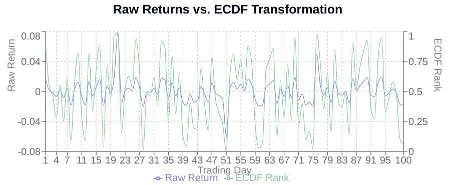
A critical innovation in the methodology is the transformation of raw returns using Empirical Cumulative Distribution Functions (ECDF). While traditional approaches directly analyze price movements, this algorithm first converts returns into their statistical ranks—creating a robust foundation less susceptible to outliers.
The implementation is elegantly concise:
self.returns = prices.pct_change().replace([np.inf, -np.inf], np.nan).ffill().dropna().to_numpy()
self.ranked_returns = np.apply_along_axis(lambda col: ECDF(col)(col), 0, self.returns)
This transformation accomplishes several mathematical objectives simultaneously:
It normalizes returns across assets with different volatility profiles.
It reduces the impact of extreme market events.
It creates a uniform statistical domain (0-1) across all assets.
It preserves the relative ordering of returns while dampening magnitude effects.