[WITH CODE] Model: Generalized Gumbel copula

Reveal the hidden dependencies that trigger extreme events

---

Table of contents:

1. Introduction.

2. Assesing limitations.

3. The copula paradigm.

4. Mathematical foundations.

5. From marginal to correlated structures.

6. The geometry of correlations.

   1. Gaussian copula.

   2. Generalized Gumbel copula.

7. The optimization trial or maximum likelihood.

---

Before you begin, remember that you have an index with the newsletter content organized by clicking on “Read the newsletter index” in this image.

---

Introduction

In quantitative finance, challenges arise when we try to model high-dimensional distributions. Let’s say you have access to abundant, high-quality univariate data—like daily returns for the SPX or the VIX—spanning 4,000 trading days. These individual time series are well understood; their empirical cumulative distribution functions are meticulously constructed using every available nuance in the data.

But here’s the catch: understanding how these variables interact is where things get tricky. Joint samples—where the returns of SPX and VIX coincide on the same day—are far scarcer, available for only about 500 days. This disparity creates a critical dilemma:

How do we preserve the rich detail of the marginal distributions while accurately modeling the underlying correlation structure with limited joint data? The answer lies in a method called copula —a framework that stitches together individual marginals with the complex dependency structures of multivariate systems.

Copulas offer a way to separate the distributional aspects from the dependence structure—a breakthrough that has transformed fields like risk management and financial engineering.

Assessing limitations

Several challenges arise when attempting to model high-dimensional distributions using copulas:

1. While univariate data is abundant, joint observations may not fully capture the dynamic interplay between variables. This scarcity raises concerns about the statistical reliability of correlation estimates.

2. Copulas excel at separating marginals from dependencies, but selecting an inappropriate parent multivariate distribution—for example, assuming a Gaussian structure when the true relationships are more complex—can lead to misestimations of tail dependencies and risk.

3. Maximum likelihood estimation, especially in high dimensions, is prone to challenges such as gradient instability and convergence issues. Factors like optimizer choice and the need for gradient clipping become critical for practical implementation.

4. As the number of variables increases, estimating the multivariate correlation matrix becomes exponentially harder. Even with modern computational tools, robust parameter estimation in higher dimensions often strains both computational resources and statistical theory.

These limitations highlight the need for careful consideration of both the data and the modeling approach.

The copula paradigm

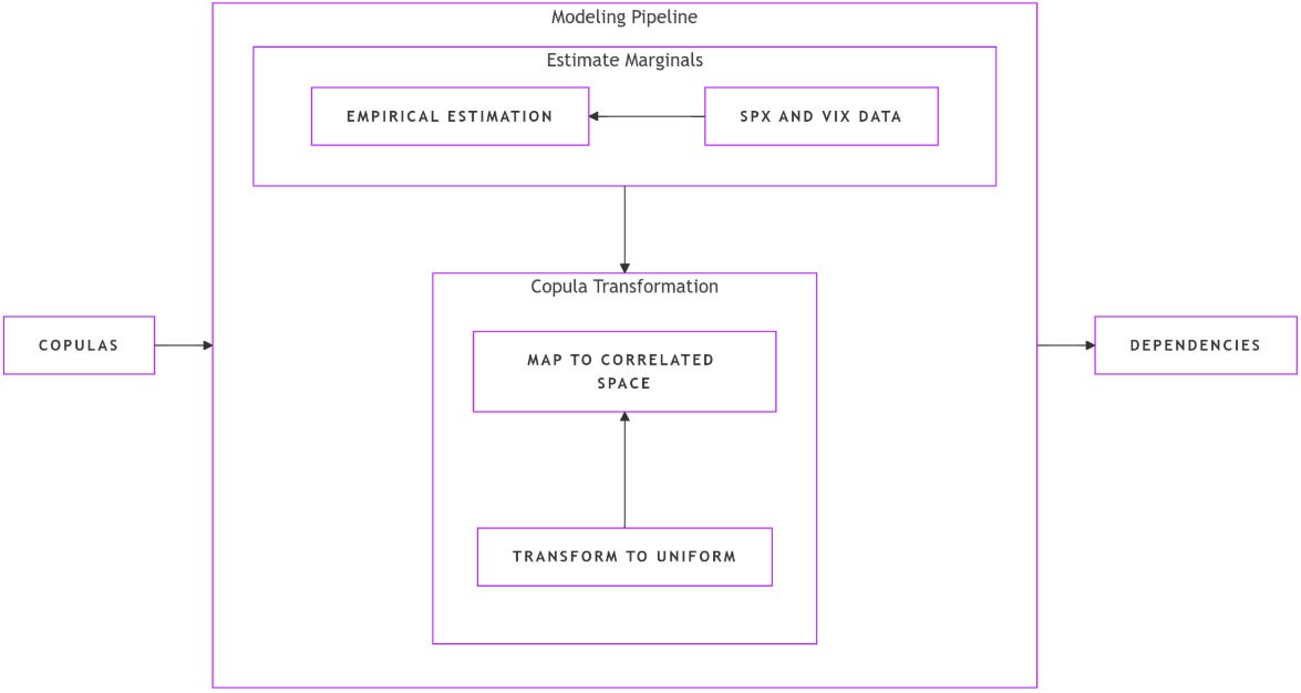
At the core of solving this problem lies the copula framework—an approach that allows us to combine univariate marginal distributions with a joint correlation structure derived from limited joint observations. Here’s how the most basic process works:

1. Constructing marginal distributions: For each variable in the system—such as SPX and VIX returns—we build robust empirical distributions. These are represented by cumulative distribution functions

   \(\phi_X(x) = \frac{1}{n} \sum I(x > X_i) \)

   derived from 4,000 samples.

2. Mapping to uniformity: The joint samples, though limited, are passed through their respective marginal CDFs to obtain values uniformly distributed in the interval [0,1]. This transformation standardizes the marginals and places the data in a copula space.

3. Reintroducing correlation through inverse transformations: Using a parent multivariate distribution, we apply the inverse CDF—quantile function—to map the uniform samples back into a space where correlations can be accurately captured.

4. Maximum likelihood estimation: Finally, MLE tunes the parameters of the parent distribution—typically the covariance matrix in the case or other parameters in generalized variants—to maximize the likelihood of the transformed joint data.

The copula framework provides a structured approach to addressing the challenge of modeling high-dimensional distributions. By separating the marginals from the dependency structure, it enables a more nuanced understanding of multivariate systems.

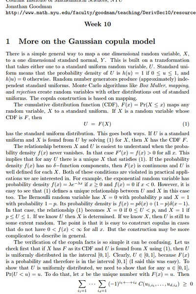
If you want to go deeper about copulas, check this:

Introduction to copulas

730KB ∙ PDF file

Download

Download

Mathematical foundations

Sklar’s Theorem provides the theoretical underpinning of this approach, stating that any multivariate joint distribution can be written in terms of its marginals and a copula that captures the dependency structure.

Consider a set of random variables {X_i,Y_i} with corresponding marginal CDFs F_X(x) and F_Y(y). The joint CDF F_X,Y(x,y) can be expressed as:

\(F_{X,Y}(x,y) = C\bigl(F_X(x), F_Y(y)\bigr)\)

where C is the copula function. This form allows quants to separately specify the individual behavior—margins—and the interdependence—copula. The elegance of this approach is its modularity. For example, in our scenario, you might have perfect estimates for F_X​ and F_Y​ derived from extensive univariate data, yet you require a method to accurately represent the joint behavior with limited joint observations.

In practical terms, one begins by transforming the joint samples into the unit hypercube. For each observation (X_i,Y_i), one computes the corresponding uniform sample:

\(U_i = F_X(X_i), \quad V_i = F_Y(Y_i)\)

These transformed values are now uniformly distributed on [0,1] and yet retain the correlation structure initially present. The next step involves lifting these uniform samples back into a space dictated by a chosen parent multivariate distribution. For instance, if we use a multivariate Gaussian as our parent distribution, we apply the inverse CDF or quantile function, denoted as

\(\phi^{-1}_{MV},\)

to each uniform sample:

\(\tilde{X}_i = \phi^{-1}_{MV}(U_i), \quad \tilde{Y}_i = \phi^{-1}_{MV}(V_i)\)

In short, the copula methodology allows us to import the detail of our high-fidelity univariate distributions into a correlated framework, much like weaving together individual threads into a coherent tapestry.

From marginal to correlated structures

The process of transitioning from independent marginal distributions to a unified, correlated multivariate structure lies at the heart of copula-based modeling. This transformation involves a systematic sequence of steps—mapping individual marginals to a standardized uniform space, then reintroducing dependencies through a chosen parent distribution.

Constructing the marginals

Begin with your individual time series. Remember we have 4,000 data points for SPX returns and VIX returns. The first step is to compute the empirical CDFs for each:

\(\phi_X(x) = \frac{1}{n} \sum_{i=1}^{n} \mathbf{1}\{X_i \le x\}\)

where 1{⋅} is the indicator function. Once these functions are built, each of the 500 joint samples (X_i,Y_i) is then transformed as:

\(u_i = \phi_X(X_i), \quad v_i = \phi_Y(Y_i)\)

This transformation ensures that both u_i​ and v_i​ are drawn from a uniform distribution over [0,1].

Transforming to the Parent distribution

Next, we assume a parent distribution—most commonly a multivariate Gaussian. In mathematical terms, if we denote the Gaussian CDF as Φ and its inverse as Φ^-1, the transformation looks like:

\(\tilde{X}_i = \Phi^{-1}(u_i), \quad \tilde{Y}_i = \Phi^{-1}(v_i)\)

In practice, this inversion maps the uniform samples back into real space, where the inherent correlation structure can be modeled with a covariance matrix Σ.

Maximum likelihood estimation and optimization

To fine-tune the model so that the parent distribution reflects the observed joint behavior, maximum likelihood estimation is employed. In many implementations, such as those using PyTorch or TensorFlow, one optimizes over the parameters of the parent distribution:

import torch as tch
import numpy as np
import matplotlib.pyplot as plt

# Covariance Calculation Function 
def tch_cov(x, rowvar=False, bias=False, ddof=None, aweights=None):
    """Estimates covariance matrix similar to numpy.cov."""
    # Ensure x is at least 2D.
    if x.dim() == 1:
        x = x.view(-1, 1)
    # Treat each column as a data point, each row as a variable.
    if rowvar and x.shape[0] != 1:
        x = x.t()
    if ddof is None:
        ddof = 1 if bias == 0 else 0
    w = aweights
    if w is not None:
        if not tch.is_tensor(w):
            w = tch.tensor(w, dtype=tch.double)
        w_sum = tch.sum(w)
        avg = tch.sum(x * (w / w_sum)[:, None], 0)
    else:
        avg = tch.mean(x, 0)
    # Determine normalization.
    fact = (x.shape[0] - ddof) if w is None else (w_sum - ddof)
    xm = x.sub(avg.expand_as(x))
    X_T = xm.t() if w is None else tch.mm(tch.diag(w), xm).t()
    c = tch.mm(X_T, xm) / fact
    return c.squeeze()

So once the covariance is computed, one might perform a Cholesky decomposition to obtain a lower triangular matrix L such that Σ=LL^T. In our Gaussian copula, maximum likelihood estimation is then used to adjust L—or, equivalently, the parameters of Σ—so that the model’s likelihood of reproducing the transformed joint data is maximized.

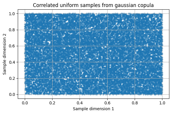
Initially, your joint samples might look like scattered points on this [0,1] square with no obvious pattern. After transformation via Φ^-1, the samples typically exhibit a structure more familiar to those who understand Gaussian behavior; clusters and ellipsoidal contours emerge—representing the latent correlation encoded in the covariance matrix.

Let’s see that:

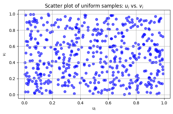
This scatter plot is​ showing uniformly distributed points. But how would we see a scatter plot after applying the inverse Gaussian CDF?

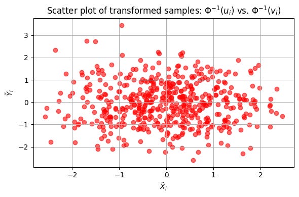
Well as you can see it is displaying a correlation structure or ellipsoidal cloud.

Such visual representations not only help validate the transformation process but also provide quantitative insight into how well the copula captures the dependency structure.

The geometry of correlations

With the fundamentals of copula construction in place, we now turn our attention to two predominant types in quantitative modeling: the Gaussian copula and the Generalized Gumbel copula.

Gaussian copula

This copula employs the multivariate normal distribution as its parent distribution. Its primary advantage lies in the intuitive appeal of using covariance as a measure of dependency. The process can be outlined as:

1. Transformation to uniform space: As described earlier, each joint sample (X_i,Y_i) is converted into (u_i,v_i) using the marginal CDFs.

2. Inverse mapping: The transformation

   \(\tilde{x}_i = \Phi^{-1}(u_i)x~i​=Φ−1(ui​) \text{ and } \tilde{y}_i = \Phi^{-1}(v_i)\)

   maps the uniform samples to a normally distributed space.

3. MLE optimization: The covariance matrix Σ is estimated using maximum likelihood estimation. This is facilitated by functions such as tch_cov and then by performing a Cholesky decomposition to ensure positive definiteness.

4. Reconstruction of correlated samples: New samples can be generated by drawing from the estimated multivariate Gaussian distribution, applying the Gaussian CDF to map them back to the unit interval, and finally using the inverse marginal CDFs to return to the original scales.

You can extend this with:

Gaussian copula

146KB ∙ PDF file

Download

Download

Okay! Then, the snippet for the Gaussian copula MLE is as follows:

# Normal CDF and Inverse CDF Functions 
def tch_normal_cdf(Y):
    return 0.5 * (1. + tch.erf(Y / np.sqrt(2.)))

def tch_normal_icdf(Y):
    return np.sqrt(2.) * tch.erfinv((2.*Y - 1.).clamp(-1 + 1e-13, 1 - 1e-13))

# Maximum Likelihood Estimation for Gaussian Copula 
def mle_gaussian_copula(Fy, analytical=False):
    """
    Estimates a Gaussian copula from empirical CDF values Fy.
    Fy must have shape (n_samples, d), with values in [0,1].
    """
    tch.set_default_tensor_type('torch.DoubleTensor')
    dim = Fy.shape[1]
    s_inds = tch.arange(dim)
    t_inds = tch.tril_indices(dim, dim)
    txs = t_inds[0].flatten()
    tys = t_inds[1].flatten()

    # Transform empirical CDF values via the inverse Gaussian CDF.
    U = tch_normal_icdf(Fy.clamp(0., 1.))
    std_t = U.std(0)
    cov = tch_cov(U) / tch.einsum('i,j->ij', std_t, std_t)
    print("Covariance Matrix:\n", cov)
    LL = tch.linalg.cholesky(cov + 0.001 * tch.eye(dim))
    if analytical:
        sigma0 = tch.matmul(LL, LL.permute(1, 0))
        sigma0[s_inds, s_inds] = tch.ones(dim)
        L = tch.linalg.cholesky(sigma0)
        return tch.distributions.MultivariateNormal(tch.zeros(dim), scale_tril=L)
    
    # Optimize over the off-diagonal correlation parameters.
    corrs = tch.nn.Parameter(LL[txs, tys], requires_grad=True)
    params = [corrs]
    optimizer = tch.optim.Adam(params, lr=2e-3)

    def get_distribution():
        L0 = tch.zeros([dim, dim])
        L0[txs, tys] = corrs
        Sigma0 = tch.matmul(L0, L0.permute(1, 0))
        Sigma0[s_inds, s_inds] = tch.ones(dim)
        L = tch.linalg.cholesky(Sigma0)
        return tch.distributions.MultivariateNormal(tch.zeros(dim), scale_tril=L)
    
    for step in range(10000):
        optimizer.zero_grad()
        D = get_distribution()
        cy_term = D.log_prob(U)
        loss = -cy_term.mean()
        loss.backward()
        tch.nn.utils.clip_grad_norm_(params, 7.)
        optimizer.step()
        if step % 100 == 0:
            print("Step {} loss: {}".format(step, loss))
    
    return get_distribution()

This returns uniform sample data as you see here:

Bautiful! It looks like my swimming pool 🤣

While the Gaussian copula may make sense in situations where one wants to obtain a base model or where one considers that the dependence can approximate a linear correlation in the central part of the distribution, in scenarios where extreme events and asymmetry are critical—as is often the case in the analysis of the S&P500 and the VIX—it is preferable to use copulas that incorporate dependence in the tails and allow capturing the non-linearity of the observed behavior.

So now that we have a general understanding of how they work, let's review and implement one whose nature is specific to modeling queues.

Generalized Gumbel copula

While the Gaussian copula is widespread, it sometimes fails to capture the extreme tail behavior—an area of particular interest in finance. The Generalized Gumbel copula addresses this shortcoming by incorporating a fat-tail dependency structure. This variant leverages the properties of the multivariate Gumbel distribution, which can better model the likelihood of joint extreme events.

The approach for the Gumbel copula parallels that of the Gaussian, with the primary distinction being the choice of the parent distribution and the corresponding transformations. For example, the one-dimensional Gumbel CDF and its inverse are defined as:

\(F_{\text{Gumbel}}(x; \mu, \beta) = \exp\big(-\exp\big(-\frac{x-\mu}{\beta}\big)\big)\)

\(F^{-1}_{\text{Gumbel}}(u; \mu, \beta) = \mu - \beta \ln\big(-\ln(u)\big)\)

The code snippet below exemplifies key components for a Generalized Gumbel copula:

# One-Dimensional Gumbel Functions 
def gumbel_1d_cdf(samples, mu=0, beta=1):
    """
    Compute the one-dimensional Gumbel CDF.
    Clamps the standardized value and then applies the Gumbel CDF transformation.
    """
    z = ((samples - mu) / beta).clamp(-12., 12.)
    return tch.exp(-tch.exp(-z))

def gumbel_1d_icdf(samples, mu=0, beta=1):
    """
    Compute the inverse of the one-dimensional Gumbel CDF.
    """
    return -beta * tch.log(-tch.log(samples)) + mu

# Generalized Gumbel Copula Class 
class GeneralizedStandardGumbel(tch.nn.Module):
    def __init__(self, alpha, rho, thresh=1e-20):
        """
        Initializes the Generalized Gumbel copula.
        alpha: lower-triangular parameter matrix for the dependency structure.
        rho: scalar parameter for tail dependency adjustment.
        """
        super(GeneralizedStandardGumbel, self).__init__()
        self.dim = alpha.shape[0]
        t_inds = tch.triu_indices(self.dim, self.dim, 1)
        self.sftpls = tch.nn.Softplus()
        self.alpha = tch.nn.Parameter(alpha[t_inds[0], t_inds[1]])
        self.rho = tch.nn.Parameter(rho * tch.ones(1))
        self.thresh = thresh

    @property
    def alpha_(self):
        a0 = self.sftpls(self.alpha)
        alpha = tch.zeros(self.dim, self.dim)
        t_inds = tch.triu_indices(self.dim, self.dim, 1)
        alpha[t_inds[0], t_inds[1]] = a0
        # Normalize the first row.
        alpha[0] /= alpha[0].sum()
        for i in range(1, self.dim - 1):
            # Normalize recursively to enforce constraints.
            alpha[i] *= (1. - alpha[:i, i].sum()) / (alpha[i].sum())
        return alpha

    @property
    def rho_(self):
        return (tch.tanh(self.rho) + 1.) / 2.

    @property
    def one_over_rho_(self):
        return (1. + tch.exp(-2. * self.rho))

    def cdf(self, y):
        """
        Computes the multivariate Gumbel CDF for the input sample y.
        """
        emy = tch.exp(-y).clamp(self.thresh, 1e13)
        if y.dim() > 1:
            alpha__ = self.alpha_.unsqueeze(0).repeat(y.shape[0], 1, 1)
            t1a = tch.einsum('...ij,...i->...ij', alpha__, emy)
            t2a = tch.einsum('...ij,...j->...ij', alpha__, emy)
            t1 = tch.pow(t1a.clamp(self.thresh, 1./self.thresh), self.one_over_rho_)
            t2 = tch.pow(t2a.clamp(self.thresh, 1./self.thresh), self.one_over_rho_)
        else:
            t1a = tch.einsum('ij,i->ij', self.alpha_, emy)
            t2a = tch.einsum('ij,j->ij', self.alpha_, emy)
            t1 = tch.pow(t1a.clamp(self.thresh, 1./self.thresh), self.one_over_rho_)
            t2 = tch.pow(t2a.clamp(self.thresh, 1./self.thresh), self.one_over_rho_)
        return tch.exp(-tch.pow((t1+t2).clamp(self.thresh, 1./self.thresh), self.rho_).sum(-1).sum(-1)).clamp(self.thresh, 1./self.thresh)

    def log_prob(self, y):
        """
        Log probability for the Gumbel copula.
        """
        return tch.log(self.cdf(y) + self.thresh)

    def rsample(self, nsamples=8000, batch_size=8000, M=400):
        """
        Generate samples via simple rejection sampling.
        """
        accepteds = []
        sum_len_accepteds = 0
        while sum_len_accepteds < nsamples:
            proposal_D = tch.distributions.MultivariateNormal(tch.zeros(self.dim), scale_tril=tch.eye(self.dim))
            proposal = proposal_D.rsample(sample_shape=[nsamples])
            fx = M * tch.exp(proposal_D.log_prob(proposal))
            g = self.cdf(proposal)
            g_o_mf = g / fx
            uniform = tch.ones(nsamples).uniform_()
            accepted = proposal[tch.logical_and(g_o_mf > uniform, 
                                                 tch.logical_not(tch.isnan(g_o_mf).sum(-1)))]
            accepteds.append(accepted)
            sum_len_accepteds = sum(acc.shape[0] for acc in accepteds)
        return tch.cat(accepteds, 0)[:nsamples]

In this case if we visualize the output we would get something like:

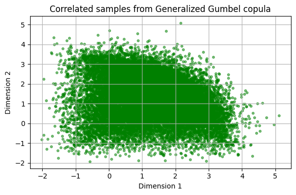
Check more about this here:

Gumbel copula

196KB ∙ PDF file

Download

Download

At this point, you're probably wondering: What's all this for?

Well, it's quite simple. We're looking to model extreme events. That's the only purpose this model would serve: how an extreme event in one asset affects another.

The optimization trial or maximum likelihood

At the heart of both copula constructions lies the art of maximum likelihood estimation. In a world replete with noise and finite samples, MLE serves as the keystone to unlock the quantitative structure hidden within the data. Whether estimating the covariance matrix for a Gaussian copula or refining the parameters of a Gumbel copula, the core idea remains: adjust the model parameters to maximize the likelihood that the model reproduces the observed—transformed—data.

In practical terms, consider the iterative process within our mle_gaussian_copula function. At each step of the optimization, the log probability of the transformed data under the current parameterization is computed. The optimizer—typically Adam—is then employed to adjust the parameters in a direction that increases this log likelihood. The loss function, defined as the negative log likelihood, is minimized over many iterations until convergence is achieved.

The mathematical formulation of the likelihood function L(θ) for our transformed data U is given by:

\(L(\theta) = \prod_{i=1}^{N} p(\tilde{x}_i, \tilde{y}_i \mid \theta)\)

where θ encapsulates the parameters of our parent distribution. Often, working with the log likelihood

\(\ell(\theta) = \sum_{i=1}^{N} \log p(\tilde{x}_i, \tilde{y}_i \mid \theta)\)

simplifies the computation and improves numerical stability. Gradient-based methods are then employed to find the optimal θ. Challenges such as vanishing or exploding gradients necessitate careful monitoring and techniques like gradient clipping, as observed in our code:

tch.nn.utils.clip_grad_norm_(params, 7.)

This single line is a safeguard, ensuring that the magnitude of the gradients does not exceed a threshold, thereby stabilizing the training process.

Let's move on to the last part - which should be part of another section, but I decided to include it here: how do we get a signal from this model?

The following two functions transform everything explained above into something understandable: 1, 0, -1 -- buy, out, sell.

For the Gaussian copula, the code would be: