[WITH CODE] Model: Queue reactive framework

Understand the dynamics of a limit order book by treating the arrivals and cancellations of orders

---

Table of contents:

1. Introduction.

2. What is the anatomy of the order book?

3. The queue reactive model.

   1. Random arrivals and Poisson processes.

   2. State-dependent intensities.

   3. Incorporating queue size effects and neighboring levels.

   4. Modeling the time until the next event.

4. Extention for the QR model.

   1. Inter-queue interactions.

   2. State-dependent intensities.

   3. Feedback loops.

---

Before you begin, remember that you have an index with the newsletter content organized by clicking on “Read full story” in this image.

---

Introduction

Picture a digital bulletin board where buyers and sellers post orders. Buyers say: I’ll pay X and sellers say: I want Y. When X and Y match, boOM!—trade happens. This board is the limit order book or LOB. It is like Tinder for stocks. Swipe right (buy) or left (sell), but everyone sees your moves.

This analogy is a little bit weird, so let's be more technical. The LOB is the engine room of modern electronic markets. It’s where all the action happens: buyers and sellers place orders, and the market continuously updates the state of play as orders are added, canceled, or executed. At its most basic level, the LOB is a ledger that contains a list of buy orders—bids—and sell orders—asks. Here’s what you need to know:

• Bid: The highest price a buyer is willing to pay for an asset.

• Ask: The lowest price a seller is willing to accept.

• Spread: The difference between the best bid and the best ask. This gap is often referred to as the “no man’s land” where prices hover until someone bridges it.

• Queue: At each price level, orders are lined up in a “first-in, first-out” (FIFO) fashion. That’s why the timing of your order placement can be as important as the price you set.

If you want more information on this topic, be sure to visit this post:

You’re the liquidity—and they’re hunting you

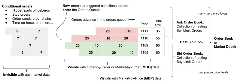
What is the anatomy of the order book?

Think of the order book like a busy restaurant’s waiting list. When you call in a reservation—place a limit order—you get in line with everyone else. The sooner you call, the better your chances of being seated at the best table—getting executed at your desired price.

The LOB is the real-time ledger of buy and sell orders in an electronic market. It isn’t just a static list; it’s a living, breathing entity that reflects market sentiment and liquidity at every moment. Here are some key points:

• Price levels and depth: Each price level has a queue of orders waiting to be executed. The depth refers to the volume available at each price. A deep book means plenty of orders—liquidity—while a shallow book can lead to larger price jumps when orders are executed.

• Bid, ask, and spread:

  • Bid: The highest price buyers are willing to pay.

  • Ask: The lowest price sellers will accept.

  • Spread: The gap between the best bid and best ask. A narrow spread is usually a sign of high liquidity.

• Order priority or FIFO:
  Orders placed at the same price are typically executed on a first-in, first-out basis. The timing of your order placement matters—a bit like arriving early for a popular concert!

Okay, first-in, first-out… easy, right? Well, not so fast. It seems simple, but in simplicity lies complexity. There's actually a lot more to it, but for the sake of this article, let's focus on what we've been discussing for now and what's represented in this image:

Let's pause for a moment on this point because it will determine your trading approach. FIFO is the default method used by brokers for managing trades, particularly when selling shares or assets. Here's how it works and the role of share quantities:

1. Standard approach:

   • Brokers typically sell the oldest purchased lots first—earliest shares acquired are sold first—unless the trader explicitly specifies otherwise—e.g., selecting specific lots.

   • This applies regardless of the number of shares traded. For example, if you bought 100 shares in January and 100 shares in March, selling 50 shares would default to the January lot under FIFO.

2. Impact of share quantities :

   • The amount of shares bought (e.g., multiple lots at different times/prices) influences which lots are prioritized under FIFO, but the method itself remains unchanged.

   • Larger sell orders involve selling shares from multiple older lots sequentially until the total quantity is met.

3. Exceptions and alternatives :

   • Traders can override FIFO by specifying lots—e.g., selecting newer shares first for tax optimization—but brokers must default to FIFO unless explicit instructions are given.

   • LIFO or Last In, First Out is rarely used in stock trading but may apply to inventory accounting for businesse.

Now scale this to millions of traders. Orders arrive en masse, one after the other. They seem random, but there's a certain dependency that generates loops and more loops, as we'll see below. What do they consist of?

Queue reactive model

The QR model helps us understand the dynamics of a limit order book by treating the arrivals and cancellations of orders as state-dependent Poisson processes. In simpler terms, the model lets the rate at which orders arrive or get canceled depend on the current state of the queue (and even its neighbors), rather than assuming a constant rate.

1. Random arrivals and Poisson processes

   In the simplest setting, assume that the arrival of orders—either new limit orders or cancellations—follows a Poisson process. This means that:

   • The time between events is exponentially distributed.

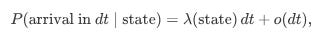
   • The probability of an event occurring in a small time interval dt is proportional to dt.

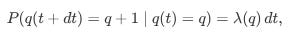
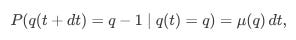
   For a small interval dt, the probability that a new limit order arrives is given by:

   

   and the probability of a cancellation is:

   

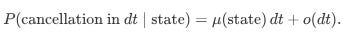
   Here, λ(state) and μ(state) are the state-dependent intensities.

   Let’s model all of this process in python to have a closer idea. First, we need to do a basic simulation of a queue with fixed arrival and service processes:

   import simpy
   import random
   import matplotlib.pyplot as plt
   
   # Simulation parameters
   RANDOM_SEED = 42
   SIM_TIME = 1000  # total simulation time
   
   def customer(env, name, counter, arrival_times, wait_times):
       """A simple customer process: records arrival time, waits for service, and then departs."""
       arrival_time = env.now
       arrival_times.append(arrival_time)
       with counter.request() as request:
           yield request
           # Service starts – calculate waiting time
           wait_time = env.now - arrival_time
           wait_times.append(wait_time)
           # Service time from an exponential distribution (mean=1)
           service_time = random.expovariate(1.0)
           yield env.timeout(service_time)
   
   def arrival_generator(env, counter, arrival_times, wait_times):
       """Generates customers with an exponential interarrival time (lambda=0.5)."""
       customer_count = 0
       while True:
           interarrival_time = random.expovariate(0.5)
           yield env.timeout(interarrival_time)
           customer_count += 1
           env.process(customer(env, f'Customer{customer_count}', counter, arrival_times, wait_times))
   
   # Setup simulation environment
   random.seed(RANDOM_SEED)
   env = simpy.Environment()
   counter = simpy.Resource(env, capacity=1)
   arrival_times = []
   wait_times = []
   
   env.process(arrival_generator(env, counter, arrival_times, wait_times))
   env.run(until=SIM_TIME)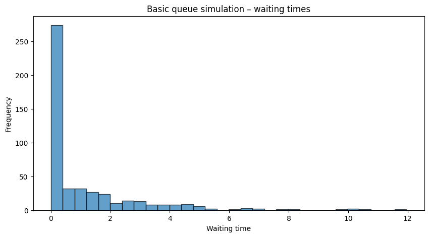

   

   Customers arrive with an exponential interarrival time, request service from a single server, and we record their waiting times.

2. State-dependent intensities

   What makes the QR Model particularly interesting is that these intensities aren’t fixed—they depend on the current state of the order book. Suppose we focus on the bid side and let q denote the number of buy orders at the best bid. We might model the intensity of new order arrivals as:

   

   and the cancellation intensity as:

   

   where:

   • α, β, γ, δ are parameters estimated from data.

   • The term βq implies that a larger queue might attract even more orders —or, in some cases, deter them if traders fear being stuck.

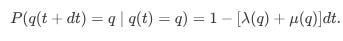
   This means that for a queue with current size q:

   • The probability of an order joining (birth) in dt is:

     

   • The probability of an order leaving (death) is:

     

   • And the probability that no event happens is:

     

   This formulation essentially models the order book as a birth-death process.

   Now, let’s introduce a reactive service mechanism that speeds up service when the queue length is high:

   def customer_reactive_service(env, name, counter, arrival_times, wait_times):
       """Customer process with a reactive service mechanism."""
       arrival_time = env.now
       arrival_times.append(arrival_time)
       with counter.request() as request:
           yield request
           wait_time = env.now - arrival_time
           wait_times.append(wait_time)
           # React based on current queue length: service speeds up if more are waiting.
           queue_length = len(counter.queue)
           base_rate = 1.0
           reactive_factor = 1 + 0.5 * queue_length  # Increase rate with queue length
           service_time = random.expovariate(base_rate * reactive_factor)
           yield env.timeout(service_time)
   
   def arrival_generator_reactive_service(env, counter, arrival_times, wait_times):
       customer_count = 0
       while True:
           interarrival_time = random.expovariate(0.5)
           yield env.timeout(interarrival_time)
           customer_count += 1
           env.process(customer_reactive_service(env, f'Customer{customer_count}', counter, arrival_times, wait_times))
   
   # Reinitialize the simulation
   random.seed(RANDOM_SEED)
   env = simpy.Environment()
   counter = simpy.Resource(env, capacity=1)
   arrival_times = []
   wait_times = []
   
   env.process(arrival_generator_reactive_service(env, counter, arrival_times, wait_times))
   env.run(until=SIM_TIME)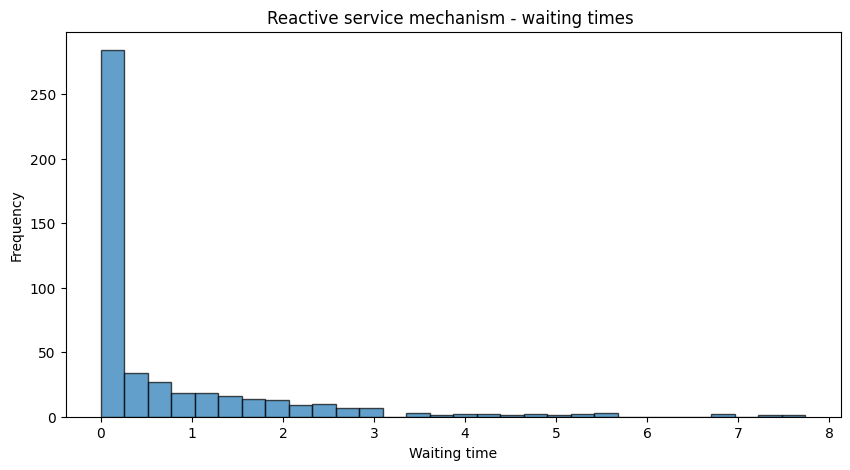

   

   Now we modify the service process so that the server “reacts” to the queue length. When more customers are waiting, the server speeds up—i.e. service rate increases—by drawing service times from a distribution whose rate parameter increases with the queue length.

3. Incorporating queue size effects and neighboring levels

   In practice, the QR Model can be extended so that the intensities depend not only on the current queue size q but also on the sizes of the neighboring queues. For example, if q_i​ is the size at level i (say, the best bid) and q_i-1​​, q_i are the sizes at the adjacent levels, then we might write:

   

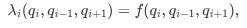
   and similarly for cancellations:

   

   This captures the feedback mechanism in the order book: a long queue might signal stability—encouraging further orders—or potential congestion—triggering cancellations—depending on the context.

   In this point, we will create a controller to adjust the arrival rate based on recent waiting times to help stabilize the system:

   def customer_reactive_service(env, name, counter, arrival_times, wait_times):
       """Customer process with reactive service mechanism (same as Part 2)."""
       arrival_time = env.now
       arrival_times.append(arrival_time)
       with counter.request() as request:
           yield request
           wait_time = env.now - arrival_time
           wait_times.append(wait_time)
           queue_length = len(counter.queue)
           base_rate = 1.0
           reactive_factor = 1 + 0.5 * queue_length
           service_time = random.expovariate(base_rate * reactive_factor)
           yield env.timeout(service_time)
   
   def arrival_generator_reactive_arrival(env, counter, arrival_times, wait_times, arrival_rate_holder):
       """Generates customers with an arrival rate that is adaptively controlled."""
       customer_count = 0
       while True:
           current_rate = arrival_rate_holder[0]
           interarrival_time = random.expovariate(current_rate)
           yield env.timeout(interarrival_time)
           customer_count += 1
           env.process(customer_reactive_service(env, f'Customer{customer_count}', counter, arrival_times, wait_times))
   
   def arrival_rate_controller(env, wait_times, arrival_rate_holder, check_interval=50, target_wait=1.0):
       """
       Periodically checks recent waiting times and adjusts the arrival rate.
       If the recent average wait exceeds the target, the arrival rate is decreased; otherwise, it is increased.
       """
       while True:
           yield env.timeout(check_interval)
           if len(wait_times) > 0:
               recent_count = min(10, len(wait_times))
               recent_avg_wait = sum(wait_times[-recent_count:]) / recent_count
               if recent_avg_wait > target_wait:
                   arrival_rate_holder[0] = max(0.1, arrival_rate_holder[0] * 0.9)
               else:
                   arrival_rate_holder[0] = arrival_rate_holder[0] * 1.1
               print(f"Time {env.now:.1f}: Adjusted arrival rate to {arrival_rate_holder[0]:.2f} (Recent avg wait: {recent_avg_wait:.2f})")
   
   # Set up simulation for reactive arrival control (without additional plots here)
   random.seed(RANDOM_SEED)
   env = simpy.Environment()
   counter = simpy.Resource(env, capacity=1)
   arrival_times = []
   wait_times = []
   arrival_rate_holder = [0.5]  # initial arrival rate
   
   env.process(arrival_generator_reactive_arrival(env, counter, arrival_times, wait_times, arrival_rate_holder))
   env.process(arrival_rate_controller(env, wait_times, arrival_rate_holder, check_interval=50, target_wait=1.0))
   env.run(until=SIM_TIME)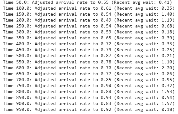

   

   A controller periodically measures recent waiting times and adjusts the arrival rate to drive the system toward a target average wait time.

4. Modeling the time until the next event

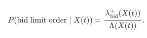
   Let the state of the order book at time t be represented by a vector X(t)—which could include q_bid​ and q_ask​ among other variables. The total intensity for any event—arrival or cancellation—is then:

   

   where superscripts “+” and “−” denote arrival and cancellation, respectively.

   The time τ until the next event is exponentially distributed with parameter Λ(X(t)):

   

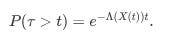
   And the probability that the next event is, for example, a bid limit order arrival is:

   

   Let’s end this part by ensambling all parts, the reactive mechanisms and a monitor process, to visualize the convergence in queue length and waiting time distributions.

   import simpy
   import random
   import matplotlib.pyplot as plt
   
   def customer_reactive(env, name, counter, arrival_times, wait_times):
       """Customer process with reactive service mechanism."""
       arrival_time = env.now
       arrival_times.append(arrival_time)
       with counter.request() as request:
           yield request
           wait_time = env.now - arrival_time
           wait_times.append(wait_time)
           # Adjust service rate based on current queue length:
           queue_length = len(counter.queue)
           base_rate = 1.0
           reactive_factor = 1 + 0.5 * queue_length
           service_time = random.expovariate(base_rate * reactive_factor)
           yield env.timeout(service_time)
   
   def arrival_generator(env, counter, arrival_times, wait_times, arrival_rate_holder):
       """Generates customers with an adaptively controlled arrival rate."""
       customer_count = 0
       while True:
           current_rate = arrival_rate_holder[0]
           interarrival_time = random.expovariate(current_rate)
           yield env.timeout(interarrival_time)
           customer_count += 1
           env.process(customer_reactive(env, f'Customer{customer_count}', counter, arrival_times, wait_times))
   
   def arrival_rate_controller(env, wait_times, arrival_rate_holder, check_interval=50, target_wait=1.0):
       """Periodically adjusts the arrival rate based on recent waiting times."""
       while True:
           yield env.timeout(check_interval)
           if len(wait_times) > 0:
               recent_count = min(10, len(wait_times))
               recent_avg_wait = sum(wait_times[-recent_count:]) / recent_count
               if recent_avg_wait > target_wait:
                   arrival_rate_holder[0] = max(0.1, arrival_rate_holder[0] * 0.9)
               else:
                   arrival_rate_holder[0] = arrival_rate_holder[0] * 1.1
               print(f"Time {env.now:.1f}: Adjusted arrival rate to {arrival_rate_holder[0]:.2f} (Recent avg wait: {recent_avg_wait:.2f})")
   
   def monitor_queue(env, counter, time_record, queue_length_record, interval=1):
       """Records the queue length at regular intervals."""
       while True:
           time_record.append(env.now)
           queue_length_record.append(len(counter.queue))
           yield env.timeout(interval)
   
   # Full simulation setup
   random.seed(RANDOM_SEED)
   env = simpy.Environment()
   counter = simpy.Resource(env, capacity=1)
   arrival_times = []
   wait_times = []
   time_record = []
   queue_length_record = []
   arrival_rate_holder = [0.5]
   
   # Start all processes: arrival generator, arrival rate controller, and queue monitor.
   env.process(arrival_generator(env, counter, arrival_times, wait_times, arrival_rate_holder))
   env.process(arrival_rate_controller(env, wait_times, arrival_rate_holder, check_interval=50, target_wait=1.0))
   env.process(monitor_queue(env, counter, time_record, queue_length_record, interval=1))
   env.run(until=SIM_TIME)
   
   # Visualization 1: Queue Length Over Time
   plt.figure(figsize=(10, 5))
   plt.plot(time_record, queue_length_record, lw=2)
   plt.xlabel('Simulation Time')
   plt.ylabel('Queue Length')
   plt.title('Queue length over time (Full QR model)')
   plt.grid(True)
   plt.show()

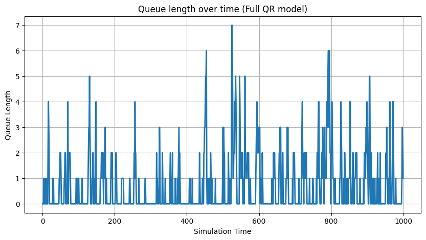
Finally, we integrate both reactive mechanisms—service and arrival—and add a monitor process that tracks the queue length over time.

Extention for the QR model

This model doesn’t stop at simple Poisson arrivals. Quants have extended the model to account for various dependencies, including:

1. Inter-queue interactions

   In a real limit order book, what happens at one price level can influence neighboring levels. For instance, if the bid side—buy orders—is very large compared to the ask side—sell orders—traders might adjust their behavior—either to join the bid or to wait before placing a sell order.

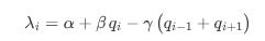
   Mathematically, the arrival intensity λ_i​ at a given price level i can be modeled as a function not only of the current queue size q_i​ but also of the sizes at adjacent levels q_i-1 and q_i+1​. One possible formulation is:

   

   Here:

   • α is a baseline arrival rate.

   • β reflects how strongly the current queue size qiq_iqi​ attracts new orders—a larger q_i​ might indicate liquidity or safety in numbers.

   • γ captures the impact of neighboring queues. A large adjacent queue—either above or below—might discourage additional orders at level i.

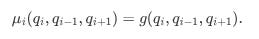
   Similarly, cancellation intensities μ_i​ might be influenced by neighboring queues:

   

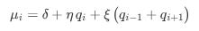
   with parameters δ, η, and ξ estimated from data.

   In a real limit order book—or in multi-class queueing systems—the arrival/cancellation rate at one queue can depend on the queue sizes at neighboring levels or classes: