

The uncertainty principle of trading
Why traditional metrics fall short, but not in the way you think


Introduction
Imagine you’re playing a game of poker. You don’t know the next card the dealer will draw, but you do know the odds of getting a flush or a straight. Trading is similar: the future is unknowable, but we can still quantify how well we’re playing the game right now.
This post isn’t about predicting the next market crash. Instead, we’ll explore how to use probability and clever metrics toreact to your trading system’s performance—in the end, isn't this what platforms like Darwinex do?
By the end, you’ll see why metrics are your financial seatbelt, not a crystal ball.
Think of this: you’re at a carnival, and a vendor offers you a magic compass that points north 60% of the time. Would you trust it? Of course not. Yet, traders often rely on metrics like the Sharpe ratio or maximum drawdown as if they’re infallible compasses in the chaotic market carnival. Let’s dissect why these tools aren’t broken—they’re just misunderstood.
Traditional metrics treat gains and losses like identical twins. But in reality, they’re more like distant cousins who only look similar. Losing $100 today means you have less capital to recover tomorrow—a mathematical death spiral most metrics ignore.
The Pitfall: Using arithmetic mean returns instead of geometric mean.
Arithmetic mean: (-10% + 10%) / 2 = 0%
Geometric mean: √(0.9 × 1.1) - 1 = -0.5%
This is what I call the symmetry trap. Check it out:
def why_arithmetic_mean_lying():
    returns = [-0.10, 0.10]
    arithmetic = np.mean(returns)
    geometric = np.prod(1 + np.array(returns)) ** (1/len(returns)) - 1
    print(f"Arithmetic Mean: {arithmetic:.2%}")  # 0.00%
    print(f"Geometric Mean: {geometric:.2%}")    # -0.50%

why_arithmetic_mean_lying() 
Why this matters? If your metric uses arithmetic mean—looking at you, Sharpe ratio. It’s like saying, “I averaged 60 mph on my road trip!” while ignoring the 3 hours you spent stuck in traffic.
Historical metrics assume the future will resemble the past—this is overfitting to calm markets!
If a strategy thrives in 2017’s low-volatility paradise, then 2020 COVID crash hits. The Sharpe ratio plummets, but by then, your portfolio is already a meme.
def sharpe_ratio(pnl):
    returns = np.diff(pnl) / pnl[:-1]
    return np.mean(returns) / np.std(returns)

# Pre-2020 data (calm markets)
pnl_peaceful = np.cumprod(1 + np.random.normal(0.001, 0.01, 100))
# Post-2020 data (chaos)
pnl_chaos = np.cumprod(1 + np.random.normal(0.001, 0.15, 100))

print(f"Pre-2020 Sharpe: {sharpe_ratio(pnl_peaceful):.2f}")  # 0.08
print(f"Post-2020 Sharpe: {sharpe_ratio(pnl_chaos):.2f}")    # -0.05
And this is the well known silent portfolio assassin. The problem?
To recover from a 20% loss, you need a 25% gain.
To recover from a 50% loss, you need a 100% gain.
Ignoring time to recover. A 50% drawdown followed by a 2-year grind back to breakeven is agony—but most metrics treat it the same as a 50% gain. Here your math proof:
Indeed, a strategy with frequent small drawdowns can be riskier than one with rare large ones. Here, a new player comes into play: volatility. You know, it is the most overrated villain in finance. Traditional metrics treat it as synonymous with risk, but volatility ≠ loss:
Strategy A: Steady 1% daily gains → Low volatility, 22% annual return.
Strategy B: Chaotic swings (-5% to +10%) → High volatility, 40% annual return.
Volatility metrics would label Strategy B as riskier, even though it makes you wealthier.
All of this leads us to the real star: the Adjusted R² metric. I admit that for a linear model, I really like this one. The linear model is the easiest path between your starting point (day 1) and your destination (final PnL). It’s the benchmark for perfect consistency.
def create_linear_model(pnl):
    n = len(pnl)
    return np.linspace(pnl[0], pnl[-1], num=n)  # Straight line from start to finish
The devil’s in the details! Residuals are the gaps between your actual PnL and the linear model. Think of them as your strategy’s mood swings:
Positive residual: You outperformed the model.
Negative residual: You underperformed.
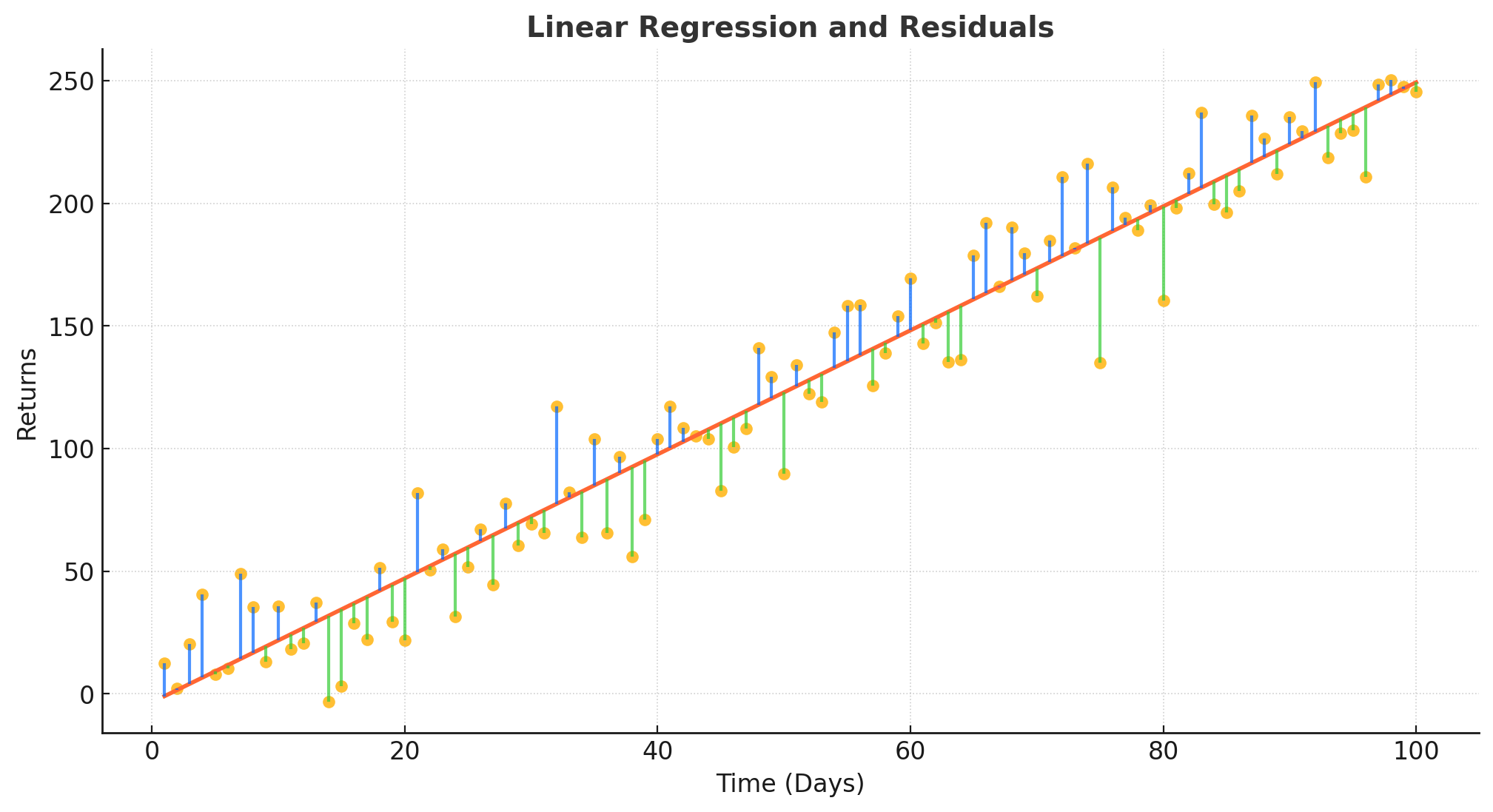
You can see how the residuals above the regression, with an acceptable fit, will always imply a growing cumulative PnL. Now, let's build a small linear model and work some magic with it to verify all this.
pnl = np.array([100, 105, 98, 110, 102])   # Toy PnL
linear = create_linear_model(pnl)          # Linear model
residuals = pnl - linear
residuals                                  # [ 0. ,  4.5, -3. ,  8.5,  0.
Oh yeah! This is where the metric gets interesting. Rather than treating all deviations the same, it penalizes losses more than it rewards gains—because losing 100 stings twice as much as winning 100 feels satisfying:
Total residual sum of squares (SS_res_total):
sum(residuals²)Negative residual sum of squares (SS_res_neg):
sum(residuals² where residuals < 0)
Why squares? Squaring residuals does two things:
Punishes large deviations disproportionately (a 10% loss isn’t 2x worse than a 5% loss—it’s 4x worse).
Ensures positivity, because negative risk scores would be weird.
I'm sure that by now you can see where I'm going. Compute the Adjusted R-squared value for a simple linear regression model where:
Since we only have PnL, we'll assume that the independent variable 𝑋 is some underlying factor. For the sake of this function, we'll assume 𝑋 is the index of the PnL series, which could represent time or another sequential factor. Being the adjusted R-squared formula:
Where:
R
²is the coefficient of determination.n is the number of observations.
k is the number of predictors (which is 1 in this case, since it's a simple linear regression).
Putting it all together. What do the previous Greek letters represent?
α (alpha): Set α > 1 to punish negative residuals extra hard.
β (beta): Set β < 1 to gently reward cumulative returns.
def adjusted_r_squared(pnl, alpha=1.2, beta=0.8, epsilon=1e-10):
    # ...[📖this is your homework for today (solved at the end)]...
    metric = 1 - (ss_res_total + alpha * ss_res_neg) / (ss_tot + beta * abs(return_cumulative))
    return np.clip(metric, 0, 1)  # Keep it between 0 and 1 (no negative scores)
How should the metric be read?
1.0: Your strategy is a gold.
0.0: Your strategy is shit.
At this point, I have another question for you: Why your strategy’s residuals aren’t normal? And why that’s okay?
Let’s play a game. Let’s say you’re at a zoo, and the zookeeper insists the unicorn exhibit is just like horses, but slightly more magical. That’s how quants describe market residuals as normally distributed. But… They’re not. They’re more like unicorns—rare, wild, and occasionally prone to setting things on fire.
The normal distribution, often called the bell curve, or My little pony of probability—comforting, predictable, and entirely mythical in trading. In reality, market residuals have fat tails, where extreme events occur far more frequently, and skewness, with losses lurking in the shadows like a horror movie villain.
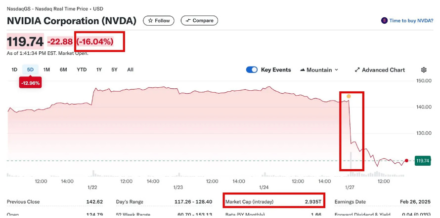
Why does this matters? If you assume residuals are normal, you’ll underestimate the risk of Black Swan events—like the battle between Deepseek and NVIDIA has given rise to a pseudo-grey swan, or whatever you want to call it.
Fat-tailed distributions are the reason your 99% safe strategy blew up last year. Let’s break it down:
Markets have more oh_$#%! moments than math textbooks admit.
Ok, and what about skewness? I've mentioned it before, but what happens with it Skewness measures how lopsided your residuals are. Negative skew = more left-tail losses—think: the 2008 housing crash. Positive skew = more right-tail gains—like finding cash in an old coat.
By punishing negative residuals with the alpha parameter, it automatically accounts for skewness. Even if your residuals resemble a deflating balloon, the metric adjusts to protect you.
Example:
Strategy A: 95% tiny gains, 5% catastrophic losses.
Strategy B: 95% tiny losses, 5% moon-shot gains.
Both might have the same average return, but Strategy A will slaughter your portfolio. The metric detects this through asymmetric penalization.
Traditional metrics throw tantrums if residuals aren’t normal. The Adjusted R² metric? It’s like a chill surfer riding any wave—normal, fat-tailed, or shaped like a dragon. How?
It uses empirical residuals—Actual historical data instead of theoretical assumptions.
It focuses on what did happen, not what should happen.
This makes it robust to:
Market crashes.
Slow-motion disasters.
By focusing on reactive metrics, you’ll survive storms and bask in sunshine. Now go forth, and may your residuals always be positive!
👍 Did you gain valuable insights and now want to empower others in the field?
Solution
def adjusted_r_squared(pnl, alpha=1.2, beta=0.8, epsilon=1e-10):
    linear = create_linear_model(pnl)
    residuals = pnl - linear
    ss_res_total = np.sum(residuals**2)
    ss_res_neg = np.sum((residuals[residuals < 0])**2)
    ss_tot = np.sum((pnl - np.mean(pnl))**2)
    return_cumulative = (pnl[-1] - pnl[0]) / (pnl[0] + epsilon)
    metric = 1 - (ss_res_total + alpha * ss_res_neg) / (ss_tot + beta * abs(return_cumulative))
    return np.clip(metric, 0, 1)