You are looking for factors
Learn how discreet factors are gradually rewriting the rules of risk and reward

Table of contents:
Introduction.
What is a factor?
Factors as building blocks of systems.
Predictive versus explanatory modeling.
Risk Factors, sparse conditions, and systematic alpha generation.
Before you begin, remember that you have an index with the newsletter content organized by clicking on “Read full story” in this image.

Introduction
The story of factor investing isn’t just a tale of numbers and models—it’s a revolution sparked in the hallowed halls of academia. Picture this: It’s the mid-20th century, and economists are on the hunt for the DNA of market success. Enter Eugene Fama and Kenneth French , two intellectual titans whose groundbreaking research didn’t just crack the code of stock returns—it rewrote it.
Fama, the University of Chicago maestro behind the Efficient Market Hypothesis, teamed up with French to dissect what really drives investment performance. Their discoveries? A set of factors acting as financial superpowers: market risk, size, value and momentum. Together, these factors formed the Fama-French model:
where:
Ri is the return of asset iii,
Rf is the risk-free rate,
αi is the asset’s alpha,
βi,1,βii,2,βii,3, are factor loadings, and
ϵi is the idiosyncratic error term.
It was a golden age and although things have changed a lot, quantitative research should be closer to the factors than to anything else.
What is a factor?
Let’s get mathematical. A factor is defined as a variable X that explains a portion of the variability in asset returns Y. The relationship is often assumed to be linear, so we model it as:
where:
Y is the asset return,
β is the sensitivity of the asset return to the factor X,
ϵ is the noise term.
In an ideal world, ϵ would be zero, but then we’d have a market as predictable as my morning coffee routine—and we all know markets are much messier than that!
But what information do you use as X? Well, there are all kinds of resources. The most common ones are:
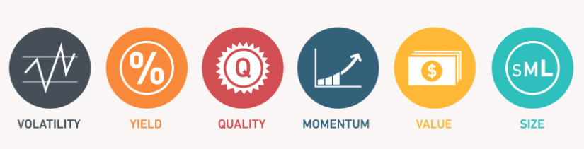
Depending on what you choose your system will produce different types of returns and risk profiles:
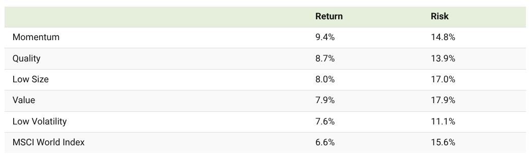
There are more. But personally I prefer high volatility factors, you will understand ahead the reason.
For the moment, the question here is: why are they so important? Factors are not just theoretical constructs—they serve as the bedrock of decision-making algorithms. But why is that!? To answer this we need to consider two key pillars:
Teleological relationships.
Causality.
Teleological relationships answer the if X then Y question. Suppose we have a factor X—say, momentum—and asset return Y. The causal hypothesis might be stated as:
But in real markets, causality is rarely so simple. Sometimes the relationship is spurious—like believing that wearing a lucky tie makes your portfolio soar. We formalize causality with the concept of conditional expectation:
where E[Y∣X] is the expected return given factor X. The challenge for quants is to differentiate between correlation and causation, and to do so with the precision of a laser-guided algorithm!
Now that we’ve warmed up with some equations, let’s journey into the factor-based approach, where the initial excitement of a novel factor quickly fades as the market catches on.
Factors as building blocks of systems
The basic building block is a factor X that informs the decision. Consider a simple strategy: if X exceeds a threshold θ, we buy; otherwise, we sell.
Mathematically, the signal S can be represented as:
The return R on the strategy might then be modeled as:
where Rj is the risk-free rate. In other words, if our factor signals buy when returns exceed the risk-free rate, we profit. But when everyone uses the same X, the signal becomes as popular as a cat video on the internet—everyone’s watching, and nothing’s new.
This could be an example of the desirable factor:
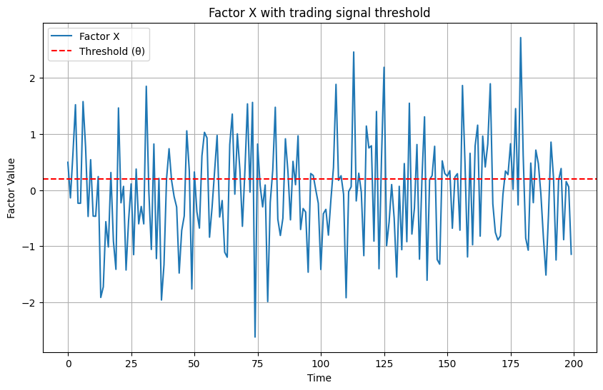
Pretty sure, huh? You'll get paid a lot of money if you find something like that.
By the way, another important issue here is factor crowding. It occurs when many market participants trade based on the same signal X. This is mathematically problematic because as more traders join the party, the effective signal strength weakens. We can describe the dilution of the factor’s effect with a crowding coefficient γ, where 0≤γ≤10:
with γ decreasing as the number of participants increases. For example, if γ=0.5, the impact of X on returns is halved compared to a less crowded market.
A neat mathematical model for crowding might look like:
where N is the number of participants and λ is a sensitivity parameter. When N is large, γ tends to zero, implying that our once-spicy factor is now as bland as unsalted oatmeal.