

[WITH CODE] Models: What are models? and algorithms?
Cracking the DNA of financial predictions and how algorithms translate market noise into signals

Table of contents:
Introduction.
What are models?
What is a logistic regression?
What is a threshold-based signal model?
What are algorithms?
How do trading models and algorithms interact?
Before you begin, remember that you have an index with the newsletter content organized by clicking on “Read full story” in this image.

Introduction
The other day, someone on X demanded to know, "What the hell does a quant actually do? And why do they get paid like they’re curing cancer or something?" My flippant reply: Magic, models, and algorithms.
But jokes aside, let’s unpack the wizardry. Quants are the financial world’s alchemists. They don’t just crunch numbers; they build crystal balls. Using advanced mathematics, machine learning, and code, they craft models that predict market movements, price derivatives, and optimize portfolios. Think of them as the architects of predictions on steroids .
And when your investments nosedive? Cue the quant-as-detective. They’re the ones sifting through terabytes of data—market ticks, economic indicators, even satellite images of parking lots—to crack the case. Why did the portfolio tank? Was it a black swan event? A flawed assumption in the risk model? A rogue algorithm? They dissect chaos like forensic scientists, turning noise into actionable insights.
As for the obscene salaries? Consider their toolkit: PhD-level expertise in stochastic calculus, coding chops to duel with AI, and the nerve to bet millions on a decimal point. They’re part mathematician, part coder, part gambler—and when they’re right, they mint money. When they’re wrong? Let’s just say you don’t want to be the one explaining that to the board.
So yeah, let's see exactly what that magic-model is.

What are models?
Think of a model as your financial GPS. It’s a simplified map of the market’s messy reality—like turning a hurricane into a breezy flowchart. Models answer: “What’s the market doing?
Basically, it is a mathematical abstraction—a simplified representation—that is used to capture essential features of market behavior. Models allow us to express complex relationships in a tractable form. They answer the question: What does the market look like?
They are the theoretical frameworks that we use to express our assumptions about how markets behave—better to have none or few. They serve as the foundation upon which trading strategies are built.
Okay, instead of assuming that returns follow a normal distribution or that the process is autoregressive, we may opt for alternative representations that better capture the reality of financial data. To illustrate this idea, let's consider these two classical models as an example:
Logistic regression.
Threshold-based signal models.
A word of caution about these models: none, I repeat, none, are going to work if you don't have the right variables 👉 Avoid price at all cost👈 Keep this in mind before plugging and playing.
What is a logistic regression?
Logistic regression is used to classify the market into distinct regimes, such as up and down states, based on a set of input variables—if you want deeper knowledge about this method, read this:

This model does not predict the magnitude of returns directly; rather, it estimates the probability that the market is in a certain regime.
We model the probability that the market is in an up regime as follows:
where:
zt is a binary indicator such that:
\(z_t = \begin{cases} 1, & \text{if the market is in an up aka buy}, \\ 0, & \text{if the market is in a down aka sell}. \end{cases}\)Xt∈Rn is a vector of explanatory variables at time t. These include measures such as momentum, volatility, volume, etc.
θ∈Rn is the parameter vector that determines the influence of each variable.
The logistic function, defined as
maps any real input x to the interval (0,1). Its derivative is given by:
This property is vital during optimization as it allows the use of gradient-based methods to adjust θ.
Well, keeping that in mind let’s code it:
import numpy as np

class LogisticRegimeModel:
    def __init__(self, theta):
        self.theta = np.array(theta)  # Parameter vector for the model

    def predict_proba(self, X):
        """
        Predicts the probability of an "up" regime given the feature matrix X.

        Parameters:
            X (np.array): Feature matrix of shape (n_samples, n_features)

        Returns:
            np.array: Probability vector with values between 0 and 1.
        """
        z = np.dot(X, self.theta)
        return 1 / (1 + np.exp(-z))

    def predict(self, X):
        """
        Classify the regime based on a threshold of 0.5.

        Parameters:
            X (np.array): Feature matrix

        Returns:
            np.array: Binary predictions where 1 indicates an up regime.
        """
        proba = self.predict_proba(X)
        return (proba >= 0.5).astype(int)

# Generate a longer example dataset
np.random.seed(42)  # For reproducibility
num_samples = 20  # Increase number of samples
X = np.random.rand(num_samples, 2) * 5  # Random values between 0 and 5

# Parameter vector (weights)
theta = np.array([0.5, -0.3])  # Coefficients for features

# Initialize the model
model = LogisticRegimeModel(theta)

# Predict probabilities
probabilities = model.predict_proba(X)
print("Predicted probabilities:", probabilities)

# Predict binary regime classification
predictions = model.predict(X)
print("Predicted regimes (0: down, 1: up):", predictions)
The output of this script is the probability:
If the probability is 0.5 or above, the market is classified as up; otherwise, it is down.
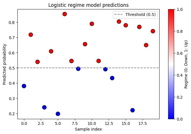
You can combine this model with the following one, as you can see there are different degrees. An output of 0.5 is not the same as one of 0.7, despite both giving the same signal: Buy!
What is a threshold-based signal model?
While logistic regression classifies the market into regimes, threshold-based models generate actionable trade signals by comparing an aggregate measure of market behavior with a threshold value—check this [Resource] for mor info about this. They serve as a non-linear mapping that translates market conditions into discrete actions, such as buy, sell, or hold.
Consider a function g(t) that represents an aggregated measure of recent feature changes. A simple formulation for g(t) is:
where:
Δft-i = ft-i-ft-i-1 is the feature change at a lag of i,
wi are weights that assign importance to each lag,
m is the number of lagged periods considered.
A discrete signal st is generated by applying a hard threshold:
where τ>0 is the threshold level.
Because hard threshold functions are not differentiable, a common approach is to use a smooth approximation such as the hyperbolic tangent:
where λ>0 controls the steepness of the transition. As λ→∞ the function approximates the hard threshold.
Let's see an example of how to implement this:
import numpy as np
import pandas as pd
import matplotlib.pyplot as plt
class ThresholdSignalModel:
def __init__(self, weights, threshold, lambda_param=10):
self.weights = np.array(weights) # Weights for lagged feature changes
self.threshold = threshold # Threshold for generating signals
self.lambda_param = lambda_param # Controls the smoothness of the tanh approximation
def compute_momentum(self, feature_series, lookback):
"""
Computes an aggregated momentum measure using lagged feature differences.
Parameters:
feature_series (pd.Series): Time series of the feature.
lookback (int): Number of periods to consider.
Returns:
pd.Series: Aggregated momentum values.
"""
feature_diff = feature_series.diff()
momentum = feature_diff.rolling(window=lookback).apply(
lambda x: np.dot(self.weights, x[-len(self.weights):]), raw=True)
return momentum
def generate_signal(self, momentum):
"""
Generates trading signals by applying a smooth threshold function.
Parameters:
momentum (pd.Series): The aggregated momentum values.
Returns:
np.array: Array of trading signals (+1, -1, or 0).
"""
smooth_signal = np.tanh(self.lambda_param * (momentum - self.threshold))
return np.where(smooth_signal > 0.5, 1, np.where(smooth_signal < -0.5, -1, 0))
# Generate synthetic volatility data
np.random.seed(42)
num_days = 100
lookback = 10
volatility_series = pd.Series(np.abs(np.random.randn(num_days) * 2)) # Simulated volatility data
# Define weights and parameters
weights = np.array([0.5, -0.3, 0.2]) # Example weights
threshold = 0.1
lookback = len(weights)
# Initialize the model
model = ThresholdSignalModel(weights, threshold)
# Compute momentum and signals using volatility instead of price
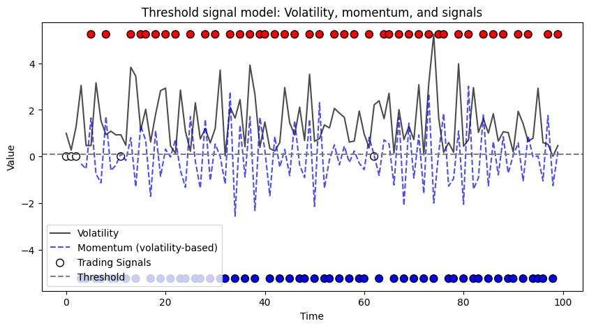
momentum_vol = model.compute_momentum(volatility_series, lookback)
signals_vol = model.generate_signal(momentum_vol)This script maps the continuous output into discrete signals: +1 for buy, -1 for sell, and 0 for no action. They are the red and blue dots —no dot? Out of the market.
Having defined what models are and provided concrete examples, we now shift our focus to algorithms—the procedures that calibrate these models and transform their outputs into trading signals.

What are algorithms?
They are the systematic processes that operationalize our mathematical models. In algorithmic trading, algorithms serve as the how in the process: how we optimize models, how we update parameters, and how we ultimately generate trading signals based on model outputs, etc.
In essence, algorithms are the workhorses that translate theoretical insights into signals—that means, the step-by-step procedures that operationalize these models.

In other words, an algorithm is a finite sequence of well-defined instructions designed to solve a specific problem. Some examples of these trading problems are:
Parameter optimization: Adjusting model parameters so that the model fits historical data well.
Signal generation: Applying the model to new data to generate actionable trade signals.
Model adaptation: Continuously updating the model as new market data arrives.
For example, one of the most widely used algorithms for optimizing model parameters is gradient descent. The fundamental idea behind gradient descent is to iteratively update parameters in the direction that minimizes a loss function.
For logistic regression, the loss function typically used is the cross-entropy loss. Given N observations
the loss is defined as:
where σ(x) is our logistic regression.
Then the gradient of L(θ) with respect to θ is computed as:
The gradient descent update rule is then given by:
where η is the learning rate that controls the step size.
May a little bit abstract, I know, but you will understand much better once it’s implemented: