[WITH CODE] Model: Combining independent signals

Why signal correlations are sabotaging your returns

---

Table of contents:

1. Introduction.

2. When one sign is not enough.

3. Noise reduction through combining independent signals.

4. Analysis of signal independence.

   1. Independence.

   2. Expectation properties and joint distributions.

   3. Covariance as a measure of dependence.

   4. Partial correlations.

5. Limits of variance reduction.

---

Introduction

Imagine driving through a city filled with intersections—each governed by a traffic light. These lights guide your way safely. Now, imagine if you had only one traffic light, and it suddenly failed. You’d likely get stuck or take a wrong turn! Trading in financial markets is quite similar. Relying on one signal to make trading decisions can be risky because that single indicator might be overwhelmed by noise or fail when market conditions change.

However, too many simultaneous and interconnected signals can cause accidents. What happens if the traffic light at an intersection is green at the same time? Your car would be like an accordion!

When one sign is not enough

Normally, one sign is not enough, but more than three could complicate traffic. Suppose we have an asset, which we label as asset i. For this asset, there are M different signals, each capturing a unique piece of market information. These signals are denoted by:

\(\quad \text{for} \quad j = 1, 2, \dots, M.\)

Each s_ij​ might represent:

• s_i1: A momentum indicator,

• s_i2: An earnings surprise measure,

• s_i3​: A volatility estimate,
  and so on.

For simplicity, we assume that these signals are already comparable—that is, they are pre-scaled to be on the same level so that we can directly average them without further normalization. Think of it as having all ingredients pre-measured for a recipe.

Once we have M comparable signals for each asset i, the next step is to combine them into a single composite signal. We define this composite signal as:

\(\alpha_{i,\text{combined}} = \sum_{j=1}^{M} w_j \, s_{ij},\)

where w_j​ is the weight assigned to the jth signal. For simplicity, we choose equal weights:

\(w_j = \frac{1}{M} \quad \text{for every } j.\)

Thus, the composite signal becomes:

\(\alpha_{i,\text{combined}} = \frac{1}{M} \sum_{j=1}^{M} s_{ij}.\)

This averaging method is our key tool for reducing noise. Even if each individual signal is noisy, their average becomes more reliable.

Now, before we go any further, I'll give you a warning about that method—and this is where the research part comes in, perhaps for later:

• The method assumes that every signal is equally reliable and informative.

• Some signals may be more predictive or less noisy than others.

• Using equal weights can lead to suboptimal results if stronger signals are diluted by weaker or less reliable ones.

• The noise reduction benefit relies on the assumption that the errors in the individual signals are uncorrelated.

• If many signals are highly correlated, the averaging process may not cancel out the noise effectively, limiting the improvement in signal quality.

• For the averaging method to work as intended, all signals must be on the same scale.

• A simple average is a linear combination, which may fail to capture nonlinear relationships between the individual signals and the asset’s behavior.

• The equal-weight scheme is static. In changing market conditions, the predictive power of individual signals might vary over time.

• A fixed average may not adjust quickly to such shifts, potentially resulting in outdated or less effective composite signals.

• If each signal contains a systematic bias, averaging them will not cancel out this bias—instead, it might reinforce it.

Since some of you have told me that sometimes you find it difficult to follow the formulations, I will give it to you already implemented.

import numpy as np

# Number of signals
M = 3

# Simulated signal values for a given asset (example)
s_i = np.array([0.5, -1.2, 0.8])  # These are s_i1, s_i2, s_i3

# Define equal weights
weights = np.ones(M) / M

# Compute the composite signal as the weighted sum
alpha_i_combined = np.dot(weights, s_i)
print("Composite signal:", alpha_i_combined)

Let’s plot these signals:

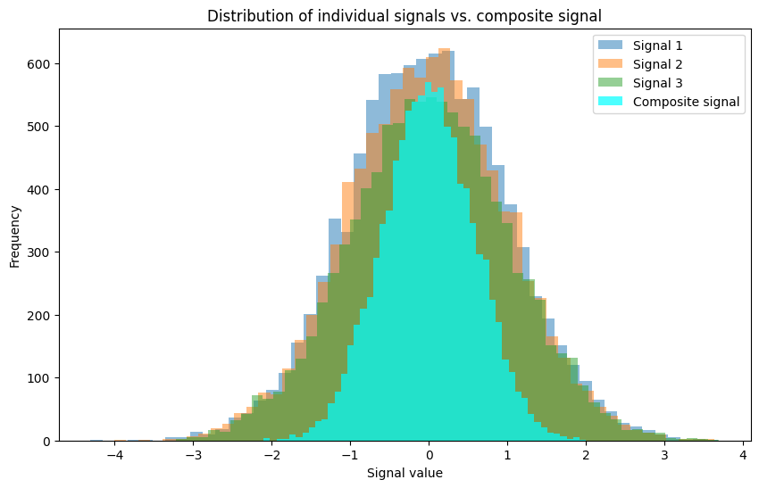
Individual signals—shown in semi-transparent colors—have a wider spread due to their noise. The composite signal—in aqua—is the average of these signals. Since the noise tends to cancel out when averaging independent variables, the composite histogram is tighter, illustrating the noise reduction benefit—if you did things right 😬

If you're curious about this method, check out this introduction to signal voting:

The science behind combining predictions

Overall, while averaging can be an effective noise reduction tool under certain conditions, careful consideration must be given to the nature of the signals—their reliability, correlations, and scales—and to the dynamics of the market environment. More sophisticated weighting methods—such as those that adjust for individual signal performance or correlation structures—might be needed to overcome these pitfalls.

Noise reduction through combining independent signals

Assume that each signal s_ij​ has a noise level quantified by its variance:

\(\operatorname{Var}(s_{ij}) = \sigma^2.\)

When the signals are independent, the variance of their sum—or average—follows a neat property. For our composite signal, we have:

\(\alpha_{i,\text{combined}} = \frac{1}{M}\sum_{j=1}^{M} s_{ij}.\)

Using the linearity of expectation and the additivity of variances for independent variables, the variance of the composite signal is:

\(\operatorname{Var}\left(\alpha_{i,\text{combined}}\right) = \operatorname{Var}\left(\frac{1}{M}\sum_{j=1}^{M} s_{ij}\right) = \frac{1}{M^2}\sum_{j=1}^{M} \operatorname{Var}(s_{ij}) = \frac{M\,\sigma^2}{M^2} = \frac{\sigma^2}{M}.\)

Thus, the noise in the composite signal is reduced by a factor of M. Even if each individual signal is noisy, their average is less noisy.

For those who appreciate a more formal mathematical treatment, consider the signals for asset iii arranged in a vector:

\(\mathbf{s}_i = \begin{pmatrix} s_{i1} \\ s_{i2} \\ \vdots \\ s_{iM} \end{pmatrix}.\)

If the signals are independent, their covariance matrix is diagonal:

\(\Sigma_i = \begin{pmatrix} \sigma^2 & 0 & \cdots & 0 \\ 0 & \sigma^2 & \cdots & 0 \\ \vdots & \vdots & \ddots & \vdots \\ 0 & 0 & \cdots & \sigma^2 \end{pmatrix}.\)

Let the weight vector be:

\(\mathbf{w} = \left(\frac{1}{M}, \frac{1}{M}, \dots, \frac{1}{M}\right)^T.\)

Then the variance of the composite signal can be written as:

\(\operatorname{Var}(\alpha_{i,\text{combined}}) = \mathbf{w}^T \Sigma_i \, \mathbf{w}.\)

Since

\(\mathbf{w}^T \Sigma_i \, \mathbf{w} = \sigma^2 \mathbf{w}^T \mathbf{w} = \sigma^2 \left(\frac{1}{M^2}\cdot M\right) = \frac{\sigma^2}{M},\)

this matrix formulation confirms our previous derivation.

import numpy as np

# Parameters
M = 3
sigma = 1.0

# Covariance matrix for independent signals (diagonal matrix)
Sigma = np.eye(M) * sigma**2

# Weight vector (equal weights)
w = np.ones(M) / M

# Compute variance of the composite signal using matrix multiplication
composite_variance = np.dot(w.T, np.dot(Sigma, w))
print("Composite signal variance (matrix formulation):", composite_variance)

The independence of the signals ensures that their covariances—off-diagonal elements—are zero, allowing for straightforward noise reduction.

Analysis of signal independence

Understanding why independence matters and how it affects the noise reduction process is crucial to appreciating the power of multiple signals.

So let’s begin by defining independence:

Two random variables X and Y are said to be independent if their joint probability distribution factorizes into the product of their individual distributions:

\(P(X = x, Y = y) = P(X = x) \cdot P(Y = y) \quad \text{for all } x, y.\)

In the context of our trading signals, this means that knowing the value of one signal does not provide any information about the other. Independence implies that the signals' noises are uncorrelated; they do not move together in a systematic way.

The mathematical definition of independence is powerful because it leads to several useful properties:

• Expectation factorization: If X and Y are independent, then:

  \(E[XY] = E[X] \cdot E[Y].\)

• Variance of the sum: For independent random variables, the variance of their sum is the sum of their variances:

  \(\operatorname{Var}(X + Y) = \operatorname{Var}(X) + \operatorname{Var}(Y).\)

These properties are the foundation for our earlier derivation showing that the variance of the composite signal is σ²/M.

Another important point here is the expectation properties and joint distributions.

Consider M independent signals s_i1,s_i2,…,s_iM​. Their joint probability distribution is given by:

\(P(s_{i1}, s_{i2}, \dots, s_{iM}) = \prod_{j=1}^{M} P(s_{ij}).\)

When calculating the expectation of the sum of these signals, the independence allows us to write:

\(E\left[\sum_{j=1}^{M} s_{ij}\right] = \sum_{j=1}^{M} E[s_{ij}].\)

If each signal is assumed to be centered—mean zero—then:

\(E[s_{ij}] = 0 \quad \text{for all } j,\)

and thus:

\(E\left[\sum_{j=1}^{M} s_{ij}\right] = 0.\)

Next, consider the expectation of the square of the composite signal:

\(E\left[\left(\frac{1}{M}\sum_{j=1}^{M} s_{ij}\right)^2\right].\)

Expanding the square, we obtain:

\(E\left[\frac{1}{M^2}\sum_{j=1}^{M}\sum_{k=1}^{M} s_{ij} s_{ik}\right].\)

Due to independence, for j≠k,

\(E[s_{ij} s_{ik}] = E[s_{ij}] E[s_{ik}] = 0.\)

Only the terms where j=k contribute:

\(E\left[\left(\frac{1}{M}\sum_{j=1}^{M} s_{ij}\right)^2\right] = \frac{1}{M^2}\sum_{j=1}^{M} E[s_{ij}^2] = \frac{1}{M^2}\cdot M\,\sigma^2 = \frac{\sigma^2}{M}.\)

Thus, the expectation properties reinforce the noise reduction result.

import numpy as np

# Parameters
M = 3
n_samples = 100000  # Using many samples for a better expectation estimate
sigma = 1.0

# Simulate independent signals from a standard normal distribution
signals = np.random.normal(0, sigma, (n_samples, M))

# Compute composite signal using equal weights
composite_signal = np.mean(signals, axis=1)

# Estimate expectation of the composite signal squared (which equals variance here, since mean ~ 0)
estimated_variance = np.mean(composite_signal**2)
print("Estimated variance of composite signal:", estimated_variance)
print("Theoretical variance (sigma^2/M):", sigma**2 / M)

But it doesn't end here, it is also possible to use covariance as a measure of dependence.

As you know, covariance is a key measure used to quantify the degree to which two random variables vary together. For two signals X and Y, the covariance is defined as:

\(\operatorname{Cov}(X, Y) = E[(X - E[X])(Y - E[Y])].\)

If X and Y are independent, then:

\(\operatorname{Cov}(X, Y) = 0.\)

This zero covariance is a necessary condition for independence—though not sufficient in all cases—and it underpins the simplifications we used earlier. For our M signals, if every pair of signals is independent, then the off-diagonal elements of the covariance matrix are all zero:

\(\Sigma_i = \begin{pmatrix} \sigma^2 & 0 & \cdots & 0 \\ 0 & \sigma^2 & \cdots & 0 \\ \vdots & \vdots & \ddots & \vdots \\ 0 & 0 & \cdots & \sigma^2 \end{pmatrix}.\)

This diagonal structure allows us to simply add variances when averaging signals:

\(\operatorname{Var}\left(\frac{1}{M}\sum_{j=1}^{M} s_{ij}\right) = \frac{1}{M^2}\sum_{j=1}^{M} \operatorname{Var}(s_{ij}) = \frac{\sigma^2}{M}.\)

import numpy as np

# Parameters
M = 3
n_samples = 1000
sigma = 1.0

# Simulate independent signals
signals = np.random.normal(0, sigma, (n_samples, M))

# Calculate the sample covariance matrix
sample_covariance = np.cov(signals, rowvar=False)
print("Sample Covariance Matrix:")
print(sample_covariance)

In the ideal case, all signals are completely independent. However, in your trading system goes life, some small correlations might exis—and here is where partial correlations come into action. Even then, if the correlations are very weak, the noise reduction benefit of averaging remains largely intact.

If we denote the correlation between any two signals s_ij​​ and s_ik—with j≠kj—as p_jk​​, then:

\(\operatorname{Cov}(s_{ij}, s_{ik}) = \rho_{jk}\,\sigma^2.\)

If p_jk​​ is close to zero, then our assumption of independence holds approximately. The variance of the composite signal then becomes:

\(\operatorname{Var}\left(\alpha_{i,\text{combined}}\right) = \frac{1}{M^2}\left(M\,\sigma^2 + \sum_{j \neq k} \rho_{jk}\,\sigma^2\right).\)

For perfect independence, all p_jk​​=0 and we recover:

\(\operatorname{Var}\left(\alpha_{i,\text{combined}}\right) = \frac{\sigma^2}{M}.\)

In many practical cases, even if the signals are not perfectly independent, as long as the average correlation is low, the noise reduction effect remains significant. This highlights why independence—or near-independence—is so valuable in constructing robust trading signals.

import numpy as np
import matplotlib.pyplot as plt

# Parameters
M = 3
n_samples = 1000
sigma = 1.0

# Simulate independent signals
signals = np.random.normal(0, sigma, (n_samples, M))

# Compute the sample correlation matrix
sample_correlation = np.corrcoef(signals, rowvar=False)
print("Sample Correlation Matrix:")
print(sample_correlation)

Limits of variance reduction

The key result we’ve derived is that for M perfectly independent signals with variance σ², the variance of the composite signal is reduced to:

\(\frac{\sigma^2}{M}.\)

This represents a significant reduction in noise. But what if the signals are not completely independent? Suppose there is some nonzero average correlation among the signals. Then the variance of the composite signal can be approximated as:

\(\operatorname{Var}\left(\alpha_{i,\text{combined}}\right) \approx \frac{1}{M^2}\left(M\,\sigma^2 + M(M-1)\,\bar{\rho}\,\sigma^2\right).\)

For small ρˉ, the reduction is still nearly σ²/M. As ρˉ​ increases, the noise reduction benefit diminishes. This expression illustrates the importance of maintaining low correlations among the signals to achieve maximum noise reduction.

It is instructive to consider extreme cases:

• Perfect independence (ρˉ=0): The variance is exactly σ²/M.

• Perfect correlation (ρˉ=1): In this case, the signals are all identical. Then:

  \(\operatorname{Var}\left(\alpha_{i,\text{combined}}\right) = \sigma^2,\)

  meaning no noise reduction is achieved by averaging.

Thus, the effectiveness of signal averaging critically depends on the degree of independence among the signals. The ideal scenario is when each signal provides unique, uncorrelated information.

Let’s see why:

import numpy as np
import matplotlib.pyplot as plt

# Parameters
M = 3
sigma = 1.0
rho_vals = np.linspace(0, 1, 100)
composite_variances = sigma**2 * (1 + (M-1)*rho_vals) / M

plt.figure(figsize=(10, 6))
plt.plot(rho_vals, composite_variances, marker='o')
plt.title("Composite signal variance vs. average correlation")
plt.xlabel("Average correlation (ρ)")
plt.ylabel("Composite variance")
plt.grid(True)
plt.show()

The output would be:

It shows that when signals are independent or ρ = 0, the composite variance is at its minimum—σ²/M. As the correlation increases, the noise reduction benefit diminishes, and when the signals are perfectly correlated or ρ = 1, no noise reduction is achieved—the composite variance equals σ². This illustrates the importance of using independent or nearly independent signals in trading systems.

Okay guys, this is all for today! Until next time—may your trades be systematic, your signals clear, and your outcomes steady. Approach the markets with math, focus, and a calm determination 💵

PS: What types of resources do you prefer for algo trading?

---

👍 Who do you know who is interested in quantitative finance and investing?

---

Appendix

Interpreted and generated signals

Interpreted and generated signals

604KB ∙ PDF file

Download

Download